Installing rethinking, Stan, and Bayesian Packages

We’ll primarily use Richard McElreath’s rethinking R package. Installation can be a bit tricky so this guide will outline how to install as well as other packages that may be helpful in this class.

`rethinking` package

The package’s github repository is the best source of information, especially the issues section where likely if you run into errors, you may find tips to help install.

Richard updated the rethinking package recently to v2.21. The biggest change is that the default Stan engine to cmdstanr instead of rstan.

Install `rstan`

While this course uses R, the engine for running Bayesian is Stan. Stan is a C++ library that can be used in a variety of ways (R, Python, Julia, Command Line, etc.).

To get started, we’ll use it with rstan, which is the R package aligned to calling Stan.

To install it, follow these instructions.

You can find more information about rstan on its website or you can view the Stan User Guide.

To test whether you properly installed rstan, try running this (see original GitHub Gist):

set.seed(123)
y <- rbinom(30, size = 1, prob = 0.2016)

y
##  [1] 0 0 0 1 1 0 0 1 0 0 1 0 0 0 0 1 0 0 0 1 1 0 0 1 0 0 0 0 0 0

# Fitting a simple binomial model using Stan
library(rstan)
## Loading required package: StanHeaders
## Loading required package: ggplot2
## rstan (Version 2.21.3, GitRev: 2e1f913d3ca3)
## For execution on a local, multicore CPU with excess RAM we recommend calling
## options(mc.cores = parallel::detectCores()).
## To avoid recompilation of unchanged Stan programs, we recommend calling
## rstan_options(auto_write = TRUE)

model_string <- "
data {
  int n;
  int y[n];
}
parameters {
  real<lower=0, upper=1> theta;
}
model {
  y ~ bernoulli(theta);
}"

stan_samples <- stan(
  model_code = model_string, 
  data = list(y = y, n = length(y)),
  seed = 123, 
  chains = 4, 
  refresh = 500
)
## 
## SAMPLING FOR MODEL 'f6f19f2978447ffaf66a6d87ed7010fd' NOW (CHAIN 1).
## Chain 1: 
## Chain 1: Gradient evaluation took 6e-06 seconds
## Chain 1: 1000 transitions using 10 leapfrog steps per transition would take 0.06 seconds.
## Chain 1: Adjust your expectations accordingly!
## Chain 1: 
## Chain 1: 
## Chain 1: Iteration:    1 / 2000 [  0%]  (Warmup)
## Chain 1: Iteration:  500 / 2000 [ 25%]  (Warmup)
## Chain 1: Iteration: 1000 / 2000 [ 50%]  (Warmup)
## Chain 1: Iteration: 1001 / 2000 [ 50%]  (Sampling)
## Chain 1: Iteration: 1500 / 2000 [ 75%]  (Sampling)
## Chain 1: Iteration: 2000 / 2000 [100%]  (Sampling)
## Chain 1: 
## Chain 1:  Elapsed Time: 0.003457 seconds (Warm-up)
## Chain 1:                0.003167 seconds (Sampling)
## Chain 1:                0.006624 seconds (Total)
## Chain 1: 
## 
## SAMPLING FOR MODEL 'f6f19f2978447ffaf66a6d87ed7010fd' NOW (CHAIN 2).
## Chain 2: 
## Chain 2: Gradient evaluation took 2e-06 seconds
## Chain 2: 1000 transitions using 10 leapfrog steps per transition would take 0.02 seconds.
## Chain 2: Adjust your expectations accordingly!
## Chain 2: 
## Chain 2: 
## Chain 2: Iteration:    1 / 2000 [  0%]  (Warmup)
## Chain 2: Iteration:  500 / 2000 [ 25%]  (Warmup)
## Chain 2: Iteration: 1000 / 2000 [ 50%]  (Warmup)
## Chain 2: Iteration: 1001 / 2000 [ 50%]  (Sampling)
## Chain 2: Iteration: 1500 / 2000 [ 75%]  (Sampling)
## Chain 2: Iteration: 2000 / 2000 [100%]  (Sampling)
## Chain 2: 
## Chain 2:  Elapsed Time: 0.003457 seconds (Warm-up)
## Chain 2:                0.003398 seconds (Sampling)
## Chain 2:                0.006855 seconds (Total)
## Chain 2: 
## 
## SAMPLING FOR MODEL 'f6f19f2978447ffaf66a6d87ed7010fd' NOW (CHAIN 3).
## Chain 3: 
## Chain 3: Gradient evaluation took 1e-06 seconds
## Chain 3: 1000 transitions using 10 leapfrog steps per transition would take 0.01 seconds.
## Chain 3: Adjust your expectations accordingly!
## Chain 3: 
## Chain 3: 
## Chain 3: Iteration:    1 / 2000 [  0%]  (Warmup)
## Chain 3: Iteration:  500 / 2000 [ 25%]  (Warmup)
## Chain 3: Iteration: 1000 / 2000 [ 50%]  (Warmup)
## Chain 3: Iteration: 1001 / 2000 [ 50%]  (Sampling)
## Chain 3: Iteration: 1500 / 2000 [ 75%]  (Sampling)
## Chain 3: Iteration: 2000 / 2000 [100%]  (Sampling)
## Chain 3: 
## Chain 3:  Elapsed Time: 0.003491 seconds (Warm-up)
## Chain 3:                0.003196 seconds (Sampling)
## Chain 3:                0.006687 seconds (Total)
## Chain 3: 
## 
## SAMPLING FOR MODEL 'f6f19f2978447ffaf66a6d87ed7010fd' NOW (CHAIN 4).
## Chain 4: 
## Chain 4: Gradient evaluation took 2e-06 seconds
## Chain 4: 1000 transitions using 10 leapfrog steps per transition would take 0.02 seconds.
## Chain 4: Adjust your expectations accordingly!
## Chain 4: 
## Chain 4: 
## Chain 4: Iteration:    1 / 2000 [  0%]  (Warmup)
## Chain 4: Iteration:  500 / 2000 [ 25%]  (Warmup)
## Chain 4: Iteration: 1000 / 2000 [ 50%]  (Warmup)
## Chain 4: Iteration: 1001 / 2000 [ 50%]  (Sampling)
## Chain 4: Iteration: 1500 / 2000 [ 75%]  (Sampling)
## Chain 4: Iteration: 2000 / 2000 [100%]  (Sampling)
## Chain 4: 
## Chain 4:  Elapsed Time: 0.003462 seconds (Warm-up)
## Chain 4:                0.003306 seconds (Sampling)
## Chain 4:                0.006768 seconds (Total)
## Chain 4:

stan_samples
## Inference for Stan model: f6f19f2978447ffaf66a6d87ed7010fd.
## 4 chains, each with iter=2000; warmup=1000; thin=1; 
## post-warmup draws per chain=1000, total post-warmup draws=4000.
## 
##         mean se_mean   sd   2.5%    25%    50%    75%  97.5% n_eff Rhat
## theta   0.28    0.00 0.08   0.14   0.22   0.27   0.33   0.45  1533    1
## lp__  -19.56    0.02 0.78 -21.77 -19.74 -19.26 -19.07 -19.01  1344    1
## 
## Samples were drawn using NUTS(diag_e) at Fri Jan  7 10:29:15 2022.
## For each parameter, n_eff is a crude measure of effective sample size,
## and Rhat is the potential scale reduction factor on split chains (at 
## convergence, Rhat=1).

traceplot(stan_samples)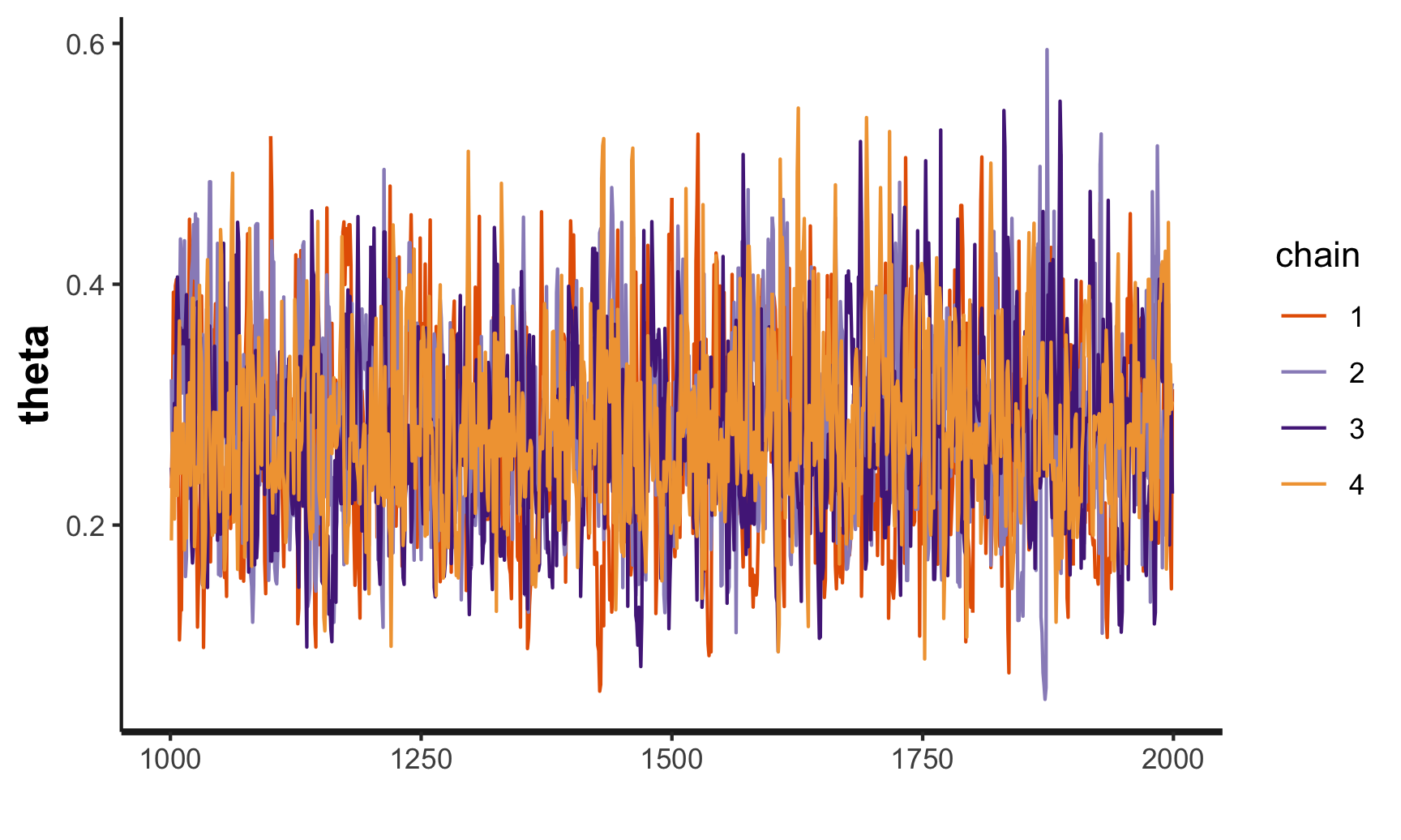

plot(stan_samples)
## ci_level: 0.8 (80% intervals)
## outer_level: 0.95 (95% intervals)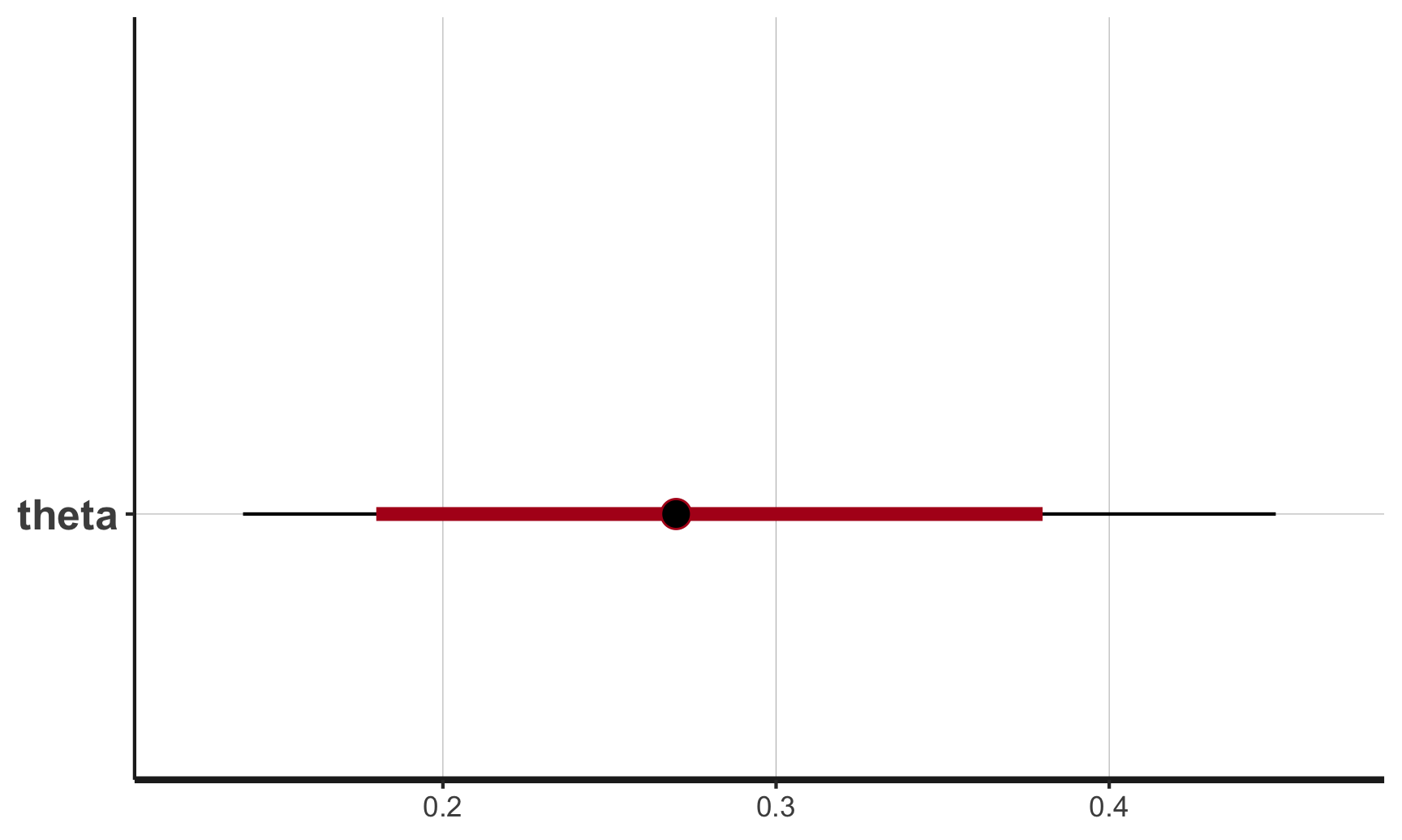

Did you get similar output?

Install `cmdstanr`

Like all things, Stan is going through changes and moving forward, rstan is falling out of favor and instead much more development will be used with cmdstanr rather than rstan (here’s a comparison).

The rethinking package works with either of these packages but it’s likely much better to use cmdstanr instead of stanr; therefore, Richard (and I) recommend installing both. https://mc-stan.org/cmdstanr/

To install cmdstanr, you’ll need to install that from github (non-CRAN library).

# if you get an error, do you have devtools installed? 
devtools::install_github("stan-dev/cmdstanr")

After you’ve installed it, if it’s your first time you’ll need to run:

# see https://mc-stan.org/cmdstanr/reference/install_cmdstan.html
cmdstanr::install_cmdstan()

To check if it was installed correctly, run:

cmdstanr::check_cmdstan_toolchain()
## The C++ toolchain required for CmdStan is setup properly!

library(cmdstanr)
## This is cmdstanr version 0.4.0.9001
## - CmdStanR documentation and vignettes: mc-stan.org/cmdstanr
## - CmdStan path: /Users/rhymenoceros/.cmdstan/cmdstan-2.28.2
## - CmdStan version: 2.28.2

file <- file.path(cmdstan_path(), "examples", "bernoulli", "bernoulli.stan")

mod <- cmdstan_model(file)
fit <- mod$sample(
  data = list(y = y, N = length(y)), # recall y from earlier example
  seed = 123, 
  chains = 4, 
  parallel_chains = 4,
  refresh = 500
)
## Running MCMC with 4 parallel chains...
## 
## Chain 1 Iteration:    1 / 2000 [  0%]  (Warmup) 
## Chain 1 Iteration:  500 / 2000 [ 25%]  (Warmup) 
## Chain 1 Iteration: 1000 / 2000 [ 50%]  (Warmup) 
## Chain 1 Iteration: 1001 / 2000 [ 50%]  (Sampling) 
## Chain 1 Iteration: 1500 / 2000 [ 75%]  (Sampling) 
## Chain 1 Iteration: 2000 / 2000 [100%]  (Sampling) 
## Chain 2 Iteration:    1 / 2000 [  0%]  (Warmup) 
## Chain 2 Iteration:  500 / 2000 [ 25%]  (Warmup) 
## Chain 2 Iteration: 1000 / 2000 [ 50%]  (Warmup) 
## Chain 2 Iteration: 1001 / 2000 [ 50%]  (Sampling) 
## Chain 2 Iteration: 1500 / 2000 [ 75%]  (Sampling) 
## Chain 2 Iteration: 2000 / 2000 [100%]  (Sampling) 
## Chain 3 Iteration:    1 / 2000 [  0%]  (Warmup) 
## Chain 3 Iteration:  500 / 2000 [ 25%]  (Warmup) 
## Chain 3 Iteration: 1000 / 2000 [ 50%]  (Warmup) 
## Chain 3 Iteration: 1001 / 2000 [ 50%]  (Sampling) 
## Chain 3 Iteration: 1500 / 2000 [ 75%]  (Sampling) 
## Chain 3 Iteration: 2000 / 2000 [100%]  (Sampling) 
## Chain 4 Iteration:    1 / 2000 [  0%]  (Warmup) 
## Chain 4 Iteration:  500 / 2000 [ 25%]  (Warmup) 
## Chain 4 Iteration: 1000 / 2000 [ 50%]  (Warmup) 
## Chain 4 Iteration: 1001 / 2000 [ 50%]  (Sampling) 
## Chain 4 Iteration: 1500 / 2000 [ 75%]  (Sampling) 
## Chain 4 Iteration: 2000 / 2000 [100%]  (Sampling) 
## Chain 1 finished in 0.0 seconds.
## Chain 2 finished in 0.0 seconds.
## Chain 3 finished in 0.0 seconds.
## Chain 4 finished in 0.0 seconds.
## 
## All 4 chains finished successfully.
## Mean chain execution time: 0.0 seconds.
## Total execution time: 0.2 seconds.

fit$summary()
## # A tibble: 2 × 10
##   variable    mean  median     sd    mad      q5     q95  rhat ess_bulk ess_tail
##   <chr>      <dbl>   <dbl>  <dbl>  <dbl>   <dbl>   <dbl> <dbl>    <dbl>    <dbl>
## 1 lp__     -19.6   -19.3   0.783  0.335  -21.0   -19.0    1.00    1703.    1945.
## 2 theta      0.278   0.274 0.0800 0.0804   0.157   0.419  1.00    1541.    1505.

Install `rethinking`

Now with both rstan and cmdstanr, you can install rethinking:

install.packages(c("coda","mvtnorm","devtools","loo","dagitty"))
devtools::install_github("rmcelreath/rethinking")

We can do a few functions to check to see if rethinking was installed correctly.

library(rethinking)
## Loading required package: parallel
## rethinking (Version 2.21)
## 
## Attaching package: 'rethinking'
## The following object is masked from 'package:rstan':
## 
##     stan
## The following object is masked from 'package:stats':
## 
##     rstudent

f <- alist(
    y ~ dnorm( mu , sigma ),
    mu ~ dnorm( 0 , 10 ),
    sigma ~ dexp( 1 )
)

fit <- quap( 
    f , 
    data=list(y=c(-1,1)) , 
    start=list(mu=0,sigma=1)
)

precis(fit)
##       mean   sd  5.5% 94.5%
## mu    0.00 0.59 -0.95  0.95
## sigma 0.84 0.33  0.31  1.36

This first runs quap which uses quadratic approximation for fitting the posterior. This is what we’ll use for the first few weeks of the class before we use MCMC methods via Stan.

# as of rethinking v2.21, cmdstan=TRUE is now default; therefore not necessary
fit_stan <- ulam( f , data=list(y=c(-1,1)), cmdstan = TRUE )
## Running MCMC with 1 chain, with 1 thread(s) per chain...
## 
## Chain 1 Iteration:   1 / 1000 [  0%]  (Warmup) 
## Chain 1 Iteration: 100 / 1000 [ 10%]  (Warmup) 
## Chain 1 Iteration: 200 / 1000 [ 20%]  (Warmup) 
## Chain 1 Iteration: 300 / 1000 [ 30%]  (Warmup) 
## Chain 1 Iteration: 400 / 1000 [ 40%]  (Warmup) 
## Chain 1 Iteration: 500 / 1000 [ 50%]  (Warmup) 
## Chain 1 Iteration: 501 / 1000 [ 50%]  (Sampling) 
## Chain 1 Iteration: 600 / 1000 [ 60%]  (Sampling) 
## Chain 1 Iteration: 700 / 1000 [ 70%]  (Sampling) 
## Chain 1 Iteration: 800 / 1000 [ 80%]  (Sampling) 
## Chain 1 Iteration: 900 / 1000 [ 90%]  (Sampling) 
## Chain 1 Iteration: 1000 / 1000 [100%]  (Sampling) 
## Chain 1 finished in 0.0 seconds.
precis(fit_stan)
##         mean   sd  5.5% 94.5% n_eff Rhat4
## mu    -0.088 1.65 -2.12   2.0    65     1
## sigma  1.625 0.94  0.69   3.5    55     1

Optional but highly helpful Bayesian packages

As Stan has grown in popularity, so too has Bayesian stats and a variety of package that work well with Stan.

`rstanarm`

First, I recommend installing rstanarm

install.packages("rstanarm")

Per its helpful vignette, the goal of the rstanarm package is to make Bayesian estimation routine for the most common regression models that applied researchers use. This will enable researchers to avoid the counter-intuitiveness of the frequentist approach to probability and statistics with only minimal changes to their existing R scripts.

To test whether the package was installed correctly, try this code:

library(rstanarm)
## Loading required package: Rcpp
## This is rstanarm version 2.21.1
## - See https://mc-stan.org/rstanarm/articles/priors for changes to default priors!
## - Default priors may change, so it's safest to specify priors, even if equivalent to the defaults.
## - For execution on a local, multicore CPU with excess RAM we recommend calling
##   options(mc.cores = parallel::detectCores())
## 
## Attaching package: 'rstanarm'
## The following objects are masked from 'package:rethinking':
## 
##     logit, se
## The following object is masked from 'package:rstan':
## 
##     loo

fit <- stan_glm(mpg ~ ., data = mtcars)
## 
## SAMPLING FOR MODEL 'continuous' NOW (CHAIN 1).
## Chain 1: 
## Chain 1: Gradient evaluation took 0.000155 seconds
## Chain 1: 1000 transitions using 10 leapfrog steps per transition would take 1.55 seconds.
## Chain 1: Adjust your expectations accordingly!
## Chain 1: 
## Chain 1: 
## Chain 1: Iteration:    1 / 2000 [  0%]  (Warmup)
## Chain 1: Iteration:  200 / 2000 [ 10%]  (Warmup)
## Chain 1: Iteration:  400 / 2000 [ 20%]  (Warmup)
## Chain 1: Iteration:  600 / 2000 [ 30%]  (Warmup)
## Chain 1: Iteration:  800 / 2000 [ 40%]  (Warmup)
## Chain 1: Iteration: 1000 / 2000 [ 50%]  (Warmup)
## Chain 1: Iteration: 1001 / 2000 [ 50%]  (Sampling)
## Chain 1: Iteration: 1200 / 2000 [ 60%]  (Sampling)
## Chain 1: Iteration: 1400 / 2000 [ 70%]  (Sampling)
## Chain 1: Iteration: 1600 / 2000 [ 80%]  (Sampling)
## Chain 1: Iteration: 1800 / 2000 [ 90%]  (Sampling)
## Chain 1: Iteration: 2000 / 2000 [100%]  (Sampling)
## Chain 1: 
## Chain 1:  Elapsed Time: 0.11012 seconds (Warm-up)
## Chain 1:                0.116468 seconds (Sampling)
## Chain 1:                0.226588 seconds (Total)
## Chain 1: 
## 
## SAMPLING FOR MODEL 'continuous' NOW (CHAIN 2).
## Chain 2: 
## Chain 2: Gradient evaluation took 4e-06 seconds
## Chain 2: 1000 transitions using 10 leapfrog steps per transition would take 0.04 seconds.
## Chain 2: Adjust your expectations accordingly!
## Chain 2: 
## Chain 2: 
## Chain 2: Iteration:    1 / 2000 [  0%]  (Warmup)
## Chain 2: Iteration:  200 / 2000 [ 10%]  (Warmup)
## Chain 2: Iteration:  400 / 2000 [ 20%]  (Warmup)
## Chain 2: Iteration:  600 / 2000 [ 30%]  (Warmup)
## Chain 2: Iteration:  800 / 2000 [ 40%]  (Warmup)
## Chain 2: Iteration: 1000 / 2000 [ 50%]  (Warmup)
## Chain 2: Iteration: 1001 / 2000 [ 50%]  (Sampling)
## Chain 2: Iteration: 1200 / 2000 [ 60%]  (Sampling)
## Chain 2: Iteration: 1400 / 2000 [ 70%]  (Sampling)
## Chain 2: Iteration: 1600 / 2000 [ 80%]  (Sampling)
## Chain 2: Iteration: 1800 / 2000 [ 90%]  (Sampling)
## Chain 2: Iteration: 2000 / 2000 [100%]  (Sampling)
## Chain 2: 
## Chain 2:  Elapsed Time: 0.104743 seconds (Warm-up)
## Chain 2:                0.089092 seconds (Sampling)
## Chain 2:                0.193835 seconds (Total)
## Chain 2: 
## 
## SAMPLING FOR MODEL 'continuous' NOW (CHAIN 3).
## Chain 3: 
## Chain 3: Gradient evaluation took 4e-06 seconds
## Chain 3: 1000 transitions using 10 leapfrog steps per transition would take 0.04 seconds.
## Chain 3: Adjust your expectations accordingly!
## Chain 3: 
## Chain 3: 
## Chain 3: Iteration:    1 / 2000 [  0%]  (Warmup)
## Chain 3: Iteration:  200 / 2000 [ 10%]  (Warmup)
## Chain 3: Iteration:  400 / 2000 [ 20%]  (Warmup)
## Chain 3: Iteration:  600 / 2000 [ 30%]  (Warmup)
## Chain 3: Iteration:  800 / 2000 [ 40%]  (Warmup)
## Chain 3: Iteration: 1000 / 2000 [ 50%]  (Warmup)
## Chain 3: Iteration: 1001 / 2000 [ 50%]  (Sampling)
## Chain 3: Iteration: 1200 / 2000 [ 60%]  (Sampling)
## Chain 3: Iteration: 1400 / 2000 [ 70%]  (Sampling)
## Chain 3: Iteration: 1600 / 2000 [ 80%]  (Sampling)
## Chain 3: Iteration: 1800 / 2000 [ 90%]  (Sampling)
## Chain 3: Iteration: 2000 / 2000 [100%]  (Sampling)
## Chain 3: 
## Chain 3:  Elapsed Time: 0.106547 seconds (Warm-up)
## Chain 3:                0.107176 seconds (Sampling)
## Chain 3:                0.213723 seconds (Total)
## Chain 3: 
## 
## SAMPLING FOR MODEL 'continuous' NOW (CHAIN 4).
## Chain 4: 
## Chain 4: Gradient evaluation took 6e-06 seconds
## Chain 4: 1000 transitions using 10 leapfrog steps per transition would take 0.06 seconds.
## Chain 4: Adjust your expectations accordingly!
## Chain 4: 
## Chain 4: 
## Chain 4: Iteration:    1 / 2000 [  0%]  (Warmup)
## Chain 4: Iteration:  200 / 2000 [ 10%]  (Warmup)
## Chain 4: Iteration:  400 / 2000 [ 20%]  (Warmup)
## Chain 4: Iteration:  600 / 2000 [ 30%]  (Warmup)
## Chain 4: Iteration:  800 / 2000 [ 40%]  (Warmup)
## Chain 4: Iteration: 1000 / 2000 [ 50%]  (Warmup)
## Chain 4: Iteration: 1001 / 2000 [ 50%]  (Sampling)
## Chain 4: Iteration: 1200 / 2000 [ 60%]  (Sampling)
## Chain 4: Iteration: 1400 / 2000 [ 70%]  (Sampling)
## Chain 4: Iteration: 1600 / 2000 [ 80%]  (Sampling)
## Chain 4: Iteration: 1800 / 2000 [ 90%]  (Sampling)
## Chain 4: Iteration: 2000 / 2000 [100%]  (Sampling)
## Chain 4: 
## Chain 4:  Elapsed Time: 0.110235 seconds (Warm-up)
## Chain 4:                0.103009 seconds (Sampling)
## Chain 4:                0.213244 seconds (Total)
## Chain 4:

plot(fit)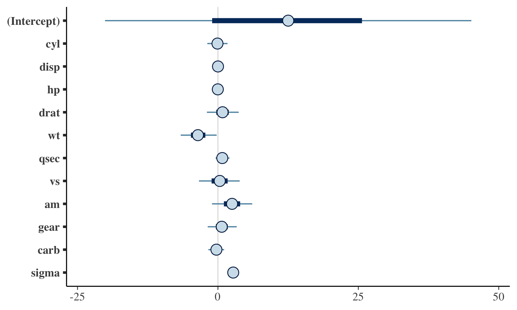

`bayesplot`

Another package that is handy is bayesplot, which provides helpful ways to visualize results from Stan models.

To install it, you’ll need to run:

install.packages("bayesplot")

You can then test it out running this code:

library(bayesplot)
## This is bayesplot version 1.8.1
## - Online documentation and vignettes at mc-stan.org/bayesplot
## - bayesplot theme set to bayesplot::theme_default()
##    * Does _not_ affect other ggplot2 plots
##    * See ?bayesplot_theme_set for details on theme setting
library(ggplot2) # assume you already have it installed

posterior <- as.matrix(fit)
plot_title <- ggtitle("Posterior distributions",
                      "with medians and 80% intervals")
mcmc_areas(posterior,
           pars = c("cyl", "drat", "am", "wt"),
           prob = 0.8) + plot_title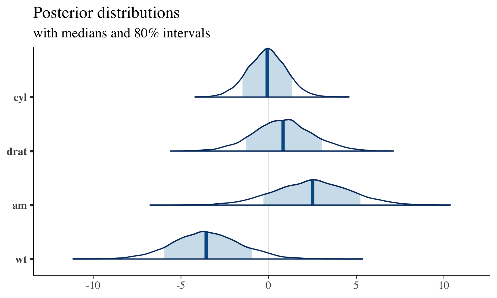

This can also provide helpful post-predictive checks (i.e., see model fitting), for example:

color_scheme_set("red")
ppc_dens_overlay(y = fit$y,
                 yrep = posterior_predict(fit, draws = 50))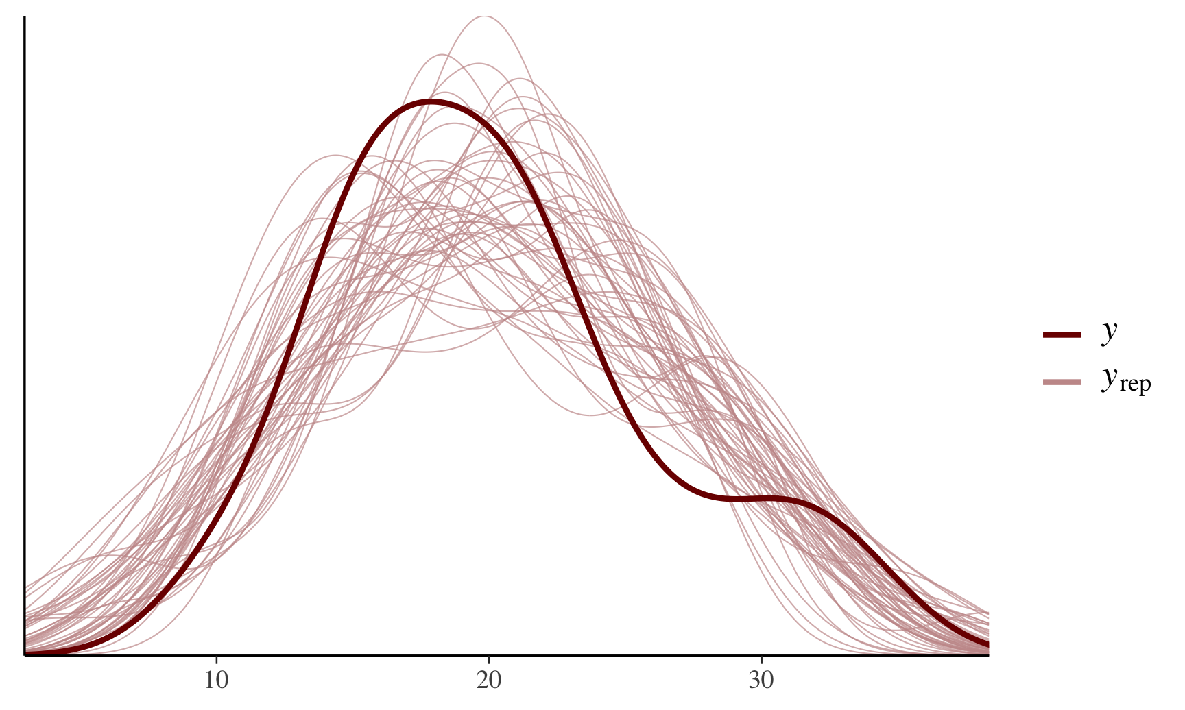

`brms`

For most Bayesian research projects, brms has become the most popular R package. https://paul-buerkner.github.io/brms/

It combines the intuition of class R regression modeling (y ~ IV1 + IV1) with mixed effects modeling like lme4 syntax. This class we won’t use this package (maybe near the end of course) but it’s incredibly helpful to think about for your final project.

Like other CRAN libraries, to install:

install.packages("brms")

You can then run Bayesian mixed effects modeling simply with:

# tidybayes example: http://mjskay.github.io/tidybayes/articles/tidy-brms.html
set.seed(5)
n = 10
n_condition = 5
ABC =
  data.frame(
    condition = rep(c("A","B","C","D","E"), n),
    response = rnorm(n * 5, c(0,1,2,1,-1), 0.5)
  )

library(brms)
## Loading 'brms' package (version 2.16.3). Useful instructions
## can be found by typing help('brms'). A more detailed introduction
## to the package is available through vignette('brms_overview').
## 
## Attaching package: 'brms'
## The following objects are masked from 'package:rstanarm':
## 
##     dirichlet, exponential, get_y, lasso, ngrps
## The following objects are masked from 'package:rethinking':
## 
##     LOO, stancode, WAIC
## The following object is masked from 'package:rstan':
## 
##     loo
## The following object is masked from 'package:stats':
## 
##     ar
m = brm(
  response ~ (1|condition), 
  data = ABC, 
  prior = c(
    prior(normal(0, 1), class = Intercept),
    prior(student_t(3, 0, 1), class = sd),
    prior(student_t(3, 0, 1), class = sigma)
  ),
  backend = "cmdstanr", # optional; if not specified, will use stanr
  control = list(adapt_delta = .99)
)
## Start sampling
## Running MCMC with 4 sequential chains...
## 
## Chain 1 Iteration:    1 / 2000 [  0%]  (Warmup) 
## Chain 1 Iteration:  100 / 2000 [  5%]  (Warmup) 
## Chain 1 Iteration:  200 / 2000 [ 10%]  (Warmup) 
## Chain 1 Iteration:  300 / 2000 [ 15%]  (Warmup) 
## Chain 1 Iteration:  400 / 2000 [ 20%]  (Warmup) 
## Chain 1 Iteration:  500 / 2000 [ 25%]  (Warmup) 
## Chain 1 Iteration:  600 / 2000 [ 30%]  (Warmup) 
## Chain 1 Iteration:  700 / 2000 [ 35%]  (Warmup) 
## Chain 1 Iteration:  800 / 2000 [ 40%]  (Warmup) 
## Chain 1 Iteration:  900 / 2000 [ 45%]  (Warmup) 
## Chain 1 Iteration: 1000 / 2000 [ 50%]  (Warmup) 
## Chain 1 Iteration: 1001 / 2000 [ 50%]  (Sampling) 
## Chain 1 Iteration: 1100 / 2000 [ 55%]  (Sampling) 
## Chain 1 Iteration: 1200 / 2000 [ 60%]  (Sampling) 
## Chain 1 Iteration: 1300 / 2000 [ 65%]  (Sampling) 
## Chain 1 Iteration: 1400 / 2000 [ 70%]  (Sampling) 
## Chain 1 Iteration: 1500 / 2000 [ 75%]  (Sampling) 
## Chain 1 Iteration: 1600 / 2000 [ 80%]  (Sampling) 
## Chain 1 Iteration: 1700 / 2000 [ 85%]  (Sampling) 
## Chain 1 Iteration: 1800 / 2000 [ 90%]  (Sampling) 
## Chain 1 Iteration: 1900 / 2000 [ 95%]  (Sampling) 
## Chain 1 Iteration: 2000 / 2000 [100%]  (Sampling) 
## Chain 1 finished in 0.4 seconds.
## Chain 2 Iteration:    1 / 2000 [  0%]  (Warmup) 
## Chain 2 Iteration:  100 / 2000 [  5%]  (Warmup) 
## Chain 2 Iteration:  200 / 2000 [ 10%]  (Warmup) 
## Chain 2 Iteration:  300 / 2000 [ 15%]  (Warmup) 
## Chain 2 Iteration:  400 / 2000 [ 20%]  (Warmup) 
## Chain 2 Iteration:  500 / 2000 [ 25%]  (Warmup) 
## Chain 2 Iteration:  600 / 2000 [ 30%]  (Warmup) 
## Chain 2 Iteration:  700 / 2000 [ 35%]  (Warmup) 
## Chain 2 Iteration:  800 / 2000 [ 40%]  (Warmup) 
## Chain 2 Iteration:  900 / 2000 [ 45%]  (Warmup) 
## Chain 2 Iteration: 1000 / 2000 [ 50%]  (Warmup) 
## Chain 2 Iteration: 1001 / 2000 [ 50%]  (Sampling) 
## Chain 2 Iteration: 1100 / 2000 [ 55%]  (Sampling) 
## Chain 2 Iteration: 1200 / 2000 [ 60%]  (Sampling) 
## Chain 2 Iteration: 1300 / 2000 [ 65%]  (Sampling) 
## Chain 2 Iteration: 1400 / 2000 [ 70%]  (Sampling) 
## Chain 2 Iteration: 1500 / 2000 [ 75%]  (Sampling) 
## Chain 2 Iteration: 1600 / 2000 [ 80%]  (Sampling) 
## Chain 2 Iteration: 1700 / 2000 [ 85%]  (Sampling) 
## Chain 2 Iteration: 1800 / 2000 [ 90%]  (Sampling) 
## Chain 2 Iteration: 1900 / 2000 [ 95%]  (Sampling) 
## Chain 2 Iteration: 2000 / 2000 [100%]  (Sampling) 
## Chain 2 finished in 0.4 seconds.
## Chain 3 Iteration:    1 / 2000 [  0%]  (Warmup) 
## Chain 3 Iteration:  100 / 2000 [  5%]  (Warmup) 
## Chain 3 Iteration:  200 / 2000 [ 10%]  (Warmup) 
## Chain 3 Iteration:  300 / 2000 [ 15%]  (Warmup) 
## Chain 3 Iteration:  400 / 2000 [ 20%]  (Warmup) 
## Chain 3 Iteration:  500 / 2000 [ 25%]  (Warmup) 
## Chain 3 Iteration:  600 / 2000 [ 30%]  (Warmup) 
## Chain 3 Iteration:  700 / 2000 [ 35%]  (Warmup) 
## Chain 3 Iteration:  800 / 2000 [ 40%]  (Warmup) 
## Chain 3 Iteration:  900 / 2000 [ 45%]  (Warmup) 
## Chain 3 Iteration: 1000 / 2000 [ 50%]  (Warmup) 
## Chain 3 Iteration: 1001 / 2000 [ 50%]  (Sampling) 
## Chain 3 Iteration: 1100 / 2000 [ 55%]  (Sampling) 
## Chain 3 Iteration: 1200 / 2000 [ 60%]  (Sampling) 
## Chain 3 Iteration: 1300 / 2000 [ 65%]  (Sampling) 
## Chain 3 Iteration: 1400 / 2000 [ 70%]  (Sampling) 
## Chain 3 Iteration: 1500 / 2000 [ 75%]  (Sampling) 
## Chain 3 Iteration: 1600 / 2000 [ 80%]  (Sampling) 
## Chain 3 Iteration: 1700 / 2000 [ 85%]  (Sampling) 
## Chain 3 Iteration: 1800 / 2000 [ 90%]  (Sampling) 
## Chain 3 Iteration: 1900 / 2000 [ 95%]  (Sampling) 
## Chain 3 Iteration: 2000 / 2000 [100%]  (Sampling) 
## Chain 3 finished in 0.5 seconds.
## Chain 4 Iteration:    1 / 2000 [  0%]  (Warmup) 
## Chain 4 Iteration:  100 / 2000 [  5%]  (Warmup) 
## Chain 4 Iteration:  200 / 2000 [ 10%]  (Warmup) 
## Chain 4 Iteration:  300 / 2000 [ 15%]  (Warmup) 
## Chain 4 Iteration:  400 / 2000 [ 20%]  (Warmup) 
## Chain 4 Iteration:  500 / 2000 [ 25%]  (Warmup) 
## Chain 4 Iteration:  600 / 2000 [ 30%]  (Warmup) 
## Chain 4 Iteration:  700 / 2000 [ 35%]  (Warmup) 
## Chain 4 Iteration:  800 / 2000 [ 40%]  (Warmup) 
## Chain 4 Iteration:  900 / 2000 [ 45%]  (Warmup) 
## Chain 4 Iteration: 1000 / 2000 [ 50%]  (Warmup) 
## Chain 4 Iteration: 1001 / 2000 [ 50%]  (Sampling) 
## Chain 4 Iteration: 1100 / 2000 [ 55%]  (Sampling) 
## Chain 4 Iteration: 1200 / 2000 [ 60%]  (Sampling) 
## Chain 4 Iteration: 1300 / 2000 [ 65%]  (Sampling) 
## Chain 4 Iteration: 1400 / 2000 [ 70%]  (Sampling) 
## Chain 4 Iteration: 1500 / 2000 [ 75%]  (Sampling) 
## Chain 4 Iteration: 1600 / 2000 [ 80%]  (Sampling) 
## Chain 4 Iteration: 1700 / 2000 [ 85%]  (Sampling) 
## Chain 4 Iteration: 1800 / 2000 [ 90%]  (Sampling) 
## Chain 4 Iteration: 1900 / 2000 [ 95%]  (Sampling) 
## Chain 4 Iteration: 2000 / 2000 [100%]  (Sampling) 
## Chain 4 finished in 0.4 seconds.
## 
## All 4 chains finished successfully.
## Mean chain execution time: 0.4 seconds.
## Total execution time: 1.8 seconds.

m
##  Family: gaussian 
##   Links: mu = identity; sigma = identity 
## Formula: response ~ (1 | condition) 
##    Data: ABC (Number of observations: 50) 
##   Draws: 4 chains, each with iter = 1000; warmup = 0; thin = 1;
##          total post-warmup draws = 4000
## 
## Group-Level Effects: 
## ~condition (Number of levels: 5) 
##               Estimate Est.Error l-95% CI u-95% CI Rhat Bulk_ESS Tail_ESS
## sd(Intercept)     1.15      0.42     0.61     2.19 1.00      890     1168
## 
## Population-Level Effects: 
##           Estimate Est.Error l-95% CI u-95% CI Rhat Bulk_ESS Tail_ESS
## Intercept     0.49      0.45    -0.46     1.36 1.00      928     1150
## 
## Family Specific Parameters: 
##       Estimate Est.Error l-95% CI u-95% CI Rhat Bulk_ESS Tail_ESS
## sigma     0.56      0.06     0.46     0.69 1.00     1700     1671
## 
## Draws were sampled using sample(hmc). For each parameter, Bulk_ESS
## and Tail_ESS are effective sample size measures, and Rhat is the potential
## scale reduction factor on split chains (at convergence, Rhat = 1).

Soloman Kurz has an amazing reproduction of our textbook but translated into brms as well as tidyverse: Statistical rethinking with brms, ggplot2, and the tidyverse: Second edition

`tidybayes` and `ggdist`

Last, tidybayes is in incredibly helpful package that combines Bayesian statistics from a tidy perspective that underpins the tidyverse.

In addition, tidybayes’ sister package, ggdist, enables incredibly powerful uncertainty visualizations via ggplot2.

To install these packages, you can run:

install.packages('ggdist')
install.packages('tidybayes')

library(ggdist)
## 
## Attaching package: 'ggdist'
## The following objects are masked from 'package:brms':
## 
##     dstudent_t, pstudent_t, qstudent_t, rstudent_t
library(tidybayes)
## 
## Attaching package: 'tidybayes'
## 
## The following objects are masked from 'package:brms':
## 
##     dstudent_t, pstudent_t, qstudent_t, rstudent_t
library(magrittr) # part of tidyverse; install if you don't have
## 
## Attaching package: 'magrittr'
## The following object is masked from 'package:rstan':
## 
##     extract
library(modelr) # install if you don't have; data_grid is from it
## 
## Attaching package: 'modelr'
## The following object is masked from 'package:rethinking':
## 
##     resample

ABC %>%
  data_grid(condition) %>%
  add_epred_rvars(m) %>%
  ggplot(aes(dist = .epred, y = condition)) +
  stat_dist_dotsinterval(quantiles = 100)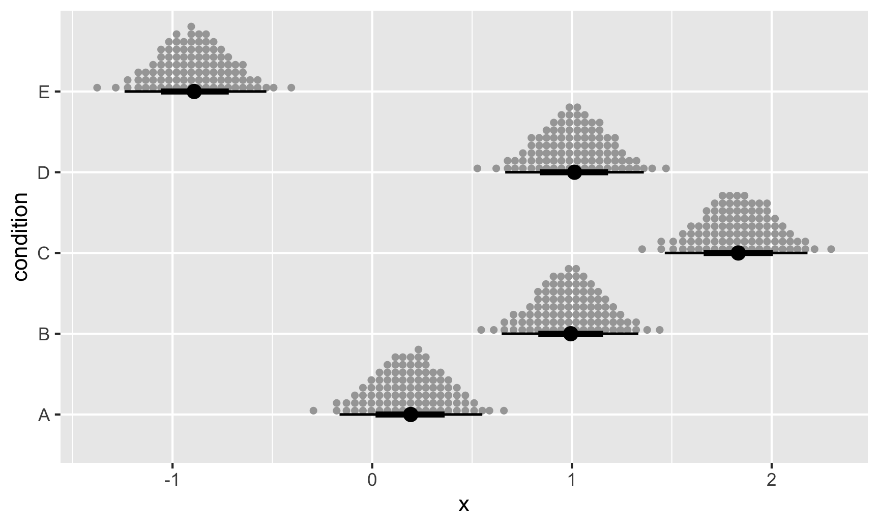

This provides posterior means using quantile dot plots, which are frequency-format uncertainty visualizations that have showed great promise in improving decision-making (Kay et al. 2016, Fernandes et al. 2018)

`tidybayes.rethinking`

There is even a tidybayes package that works specifically for the rethinking package. I encourage you to install this as we may

devtools::install_github("mjskay/tidybayes.rethinking")

You can now run this:

library(tidybayes.rethinking)

# bayesian regression wt (x) on mpg (y)
m = quap(alist(
    mpg ~ dlnorm(mu, sigma),
    mu <- a + b*wt,
    c(a,b) ~ dnorm(0, 10),
    sigma ~ dexp(1)
  ),
  data = mtcars,
  start = list(a = 4, b = -1, sigma = 1)
)

m %>%
  tidybayes::tidy_draws() %>%
  tidybayes::gather_variables() %>%
  median_qi() %>%
  ggplot(aes(y = .variable, x = .value, xmin = .lower, xmax = .upper)) +
  geom_pointinterval()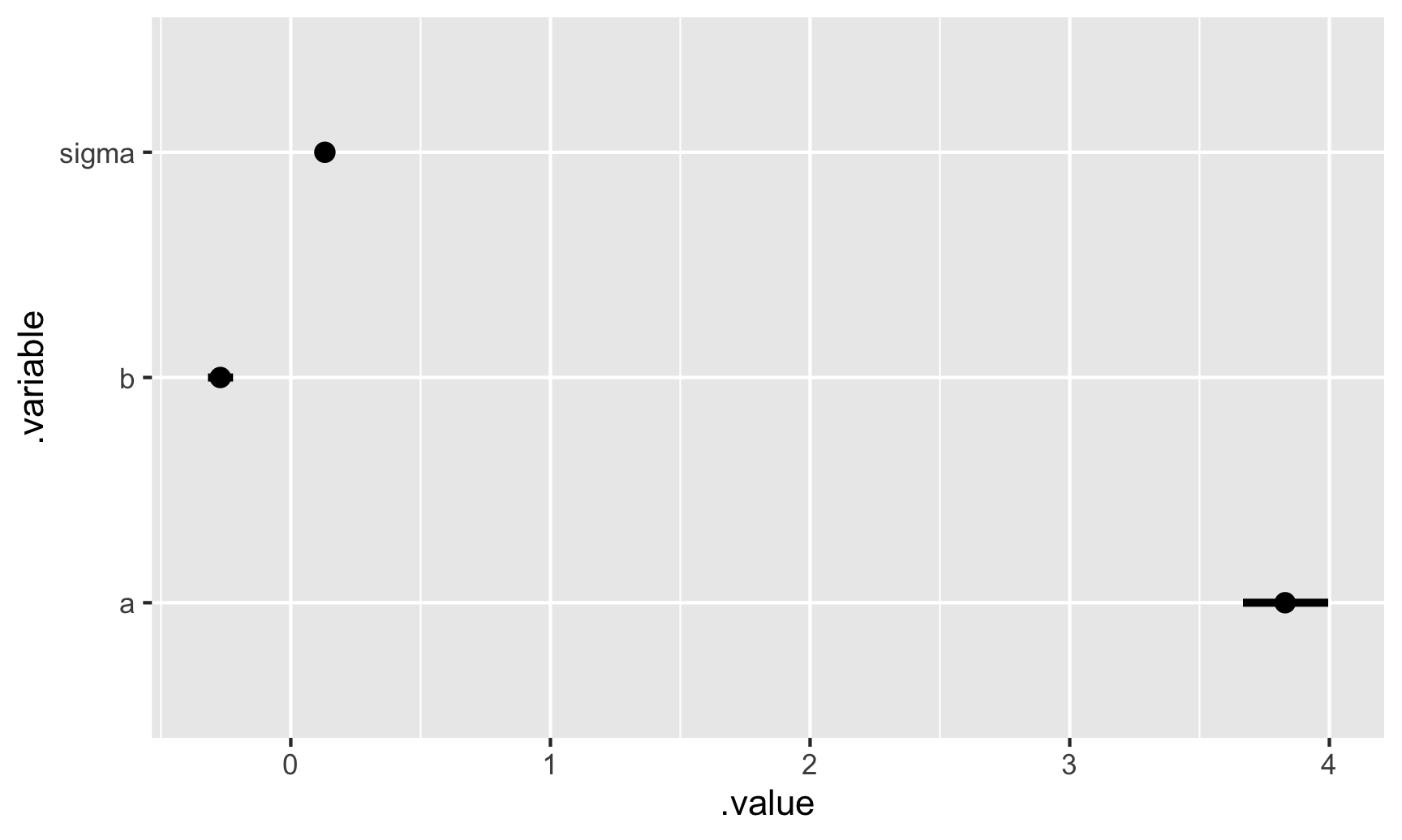

Package versions above

When using R (or any open source language), it’s very important to keep links for package versions. I highly recommend running in Rmarkdown files this code at the end to timestamp what packages were used.

sessionInfo()
## R version 4.1.1 (2021-08-10)
## Platform: aarch64-apple-darwin20 (64-bit)
## Running under: macOS Monterey 12.0.1
## 
## Matrix products: default
## BLAS:   /Library/Frameworks/R.framework/Versions/4.1-arm64/Resources/lib/libRblas.0.dylib
## LAPACK: /Library/Frameworks/R.framework/Versions/4.1-arm64/Resources/lib/libRlapack.dylib
## 
## locale:
## [1] en_US.UTF-8/en_US.UTF-8/en_US.UTF-8/C/en_US.UTF-8/en_US.UTF-8
## 
## attached base packages:
## [1] parallel  stats     graphics  grDevices datasets  utils     methods   base     
## 
## other attached packages:
##  [1] tidybayes.rethinking_3.0.0 modelr_0.1.8               magrittr_2.0.1             tidybayes_3.0.1            ggdist_3.0.1              
##  [6] brms_2.16.3                bayesplot_1.8.1            rstanarm_2.21.1            Rcpp_1.0.7                 digest_0.6.29             
## [11] rethinking_2.21            cmdstanr_0.4.0.9001        rstan_2.21.3               ggplot2_3.3.5              StanHeaders_2.21.0-7      
## 
## loaded via a namespace (and not attached):
##   [1] minqa_1.2.4          colorspace_2.0-2     ellipsis_0.3.2       ggridges_0.5.3       rsconnect_0.8.25     markdown_1.1        
##   [7] base64enc_0.1-3      xaringanExtra_0.5.5  rstudioapi_0.13      farver_2.1.0         svUnit_1.0.6         DT_0.20             
##  [13] fansi_0.5.0          mvtnorm_1.1-3        bridgesampling_1.1-2 codetools_0.2-18     splines_4.1.1        knitr_1.36          
##  [19] shinythemes_1.2.0    jsonlite_1.7.2       nloptr_1.2.2.3       broom_0.7.9          shiny_1.7.1          compiler_4.1.1      
##  [25] backports_1.4.1      assertthat_0.2.1     Matrix_1.3-4         fastmap_1.1.0        cli_3.1.0            later_1.3.0         
##  [31] htmltools_0.5.2      prettyunits_1.1.1    tools_4.1.1          igraph_1.2.9         coda_0.19-4          gtable_0.3.0        
##  [37] glue_1.6.0           reshape2_1.4.4       dplyr_1.0.7          posterior_1.1.0      jquerylib_0.1.4      vctrs_0.3.8         
##  [43] nlme_3.1-152         blogdown_1.5         crosstalk_1.2.0      tensorA_0.36.2       xfun_0.28            stringr_1.4.0       
##  [49] ps_1.6.0             lme4_1.1-27.1        mime_0.12            miniUI_0.1.1.1       lifecycle_1.0.1      renv_0.14.0         
##  [55] gtools_3.9.2         MASS_7.3-54          zoo_1.8-9            scales_1.1.1         colourpicker_1.1.1   Brobdingnag_1.2-6   
##  [61] promises_1.2.0.1     inline_0.3.19        shinystan_2.5.0      yaml_2.2.1           gridExtra_2.3        loo_2.4.1           
##  [67] sass_0.4.0           stringi_1.7.6        highr_0.9            dygraphs_1.1.1.6     checkmate_2.0.0      boot_1.3-28         
##  [73] pkgbuild_1.3.1       shape_1.4.6          rlang_0.4.12         pkgconfig_2.0.3      matrixStats_0.61.0   distributional_0.2.2
##  [79] evaluate_0.14        lattice_0.20-44      purrr_0.3.4          rstantools_2.1.1     htmlwidgets_1.5.4    labeling_0.4.2      
##  [85] processx_3.5.2       tidyselect_1.1.1     plyr_1.8.6           bookdown_0.24        R6_2.5.1             generics_0.1.1      
##  [91] DBI_1.1.1            pillar_1.6.4         withr_2.4.3          xts_0.12.1           survival_3.2-11      abind_1.4-5         
##  [97] tibble_3.1.6         crayon_1.4.2         arrayhelpers_1.1-0   uuid_1.0-3           utf8_1.2.2           rmarkdown_2.11      
## [103] grid_4.1.1           data.table_1.14.2    callr_3.7.0          threejs_0.3.3        xtable_1.8-4         tidyr_1.1.4         
## [109] httpuv_1.6.3         RcppParallel_5.1.4   stats4_4.1.1         munsell_0.5.0        bslib_0.3.1          shinyjs_2.0.0

Last updated on Jan 7, 2022

Installing rethinking, Stan, and Bayesian Packages

rethinking package

Install rstan

Install cmdstanr

Install rethinking

Optional but highly helpful Bayesian packages

rstanarm

bayesplot

brms

tidybayes and ggdist

tidybayes.rethinking