Class 15
In-Class Lab: Chapter 16
In this lab, we’ll go through two examples from Chapter 16 with models that go beyond generalized linear models.
Geometric People
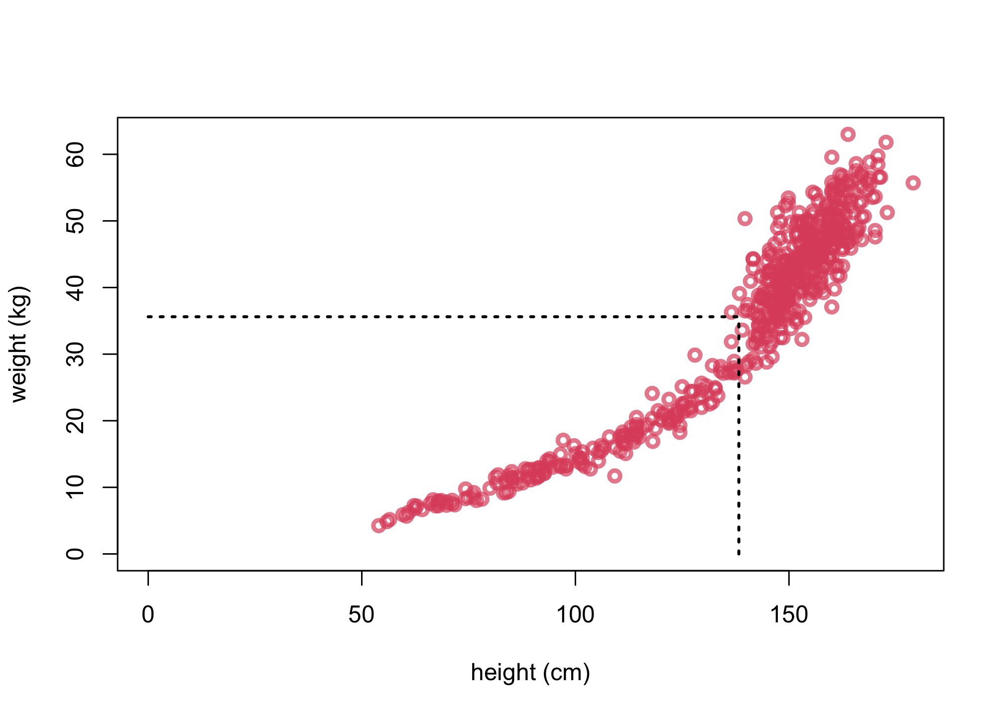
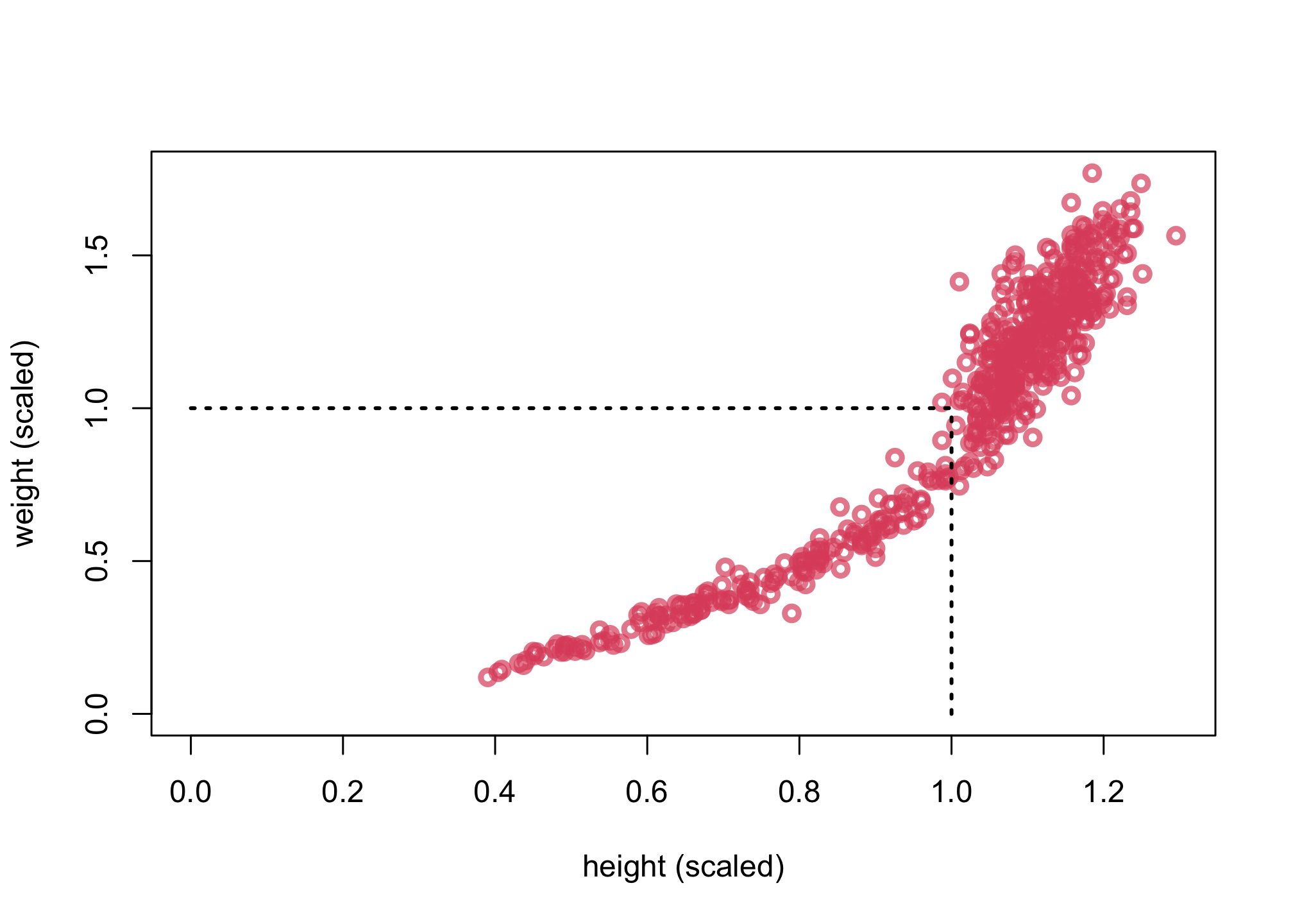
Let’s review the Howell1 dataset and scale the values per 16.1 to eliminate the units.
library(rethinking)
data(Howell1)
d <- Howell1

# scale observed variables
d$w <- d$weight / mean(d$weight)
d$h <- d$height / mean(d$height)
We can follow the code in lecture to view both plots.
plot( d$height , d$weight , xlim=c(0,max(d$height)) , ylim=c(0,max(d$weight)) , col=col.alpha(2,0.7) ,
    lwd=3 , xlab="height (cm)" , ylab="weight (kg)" )
mw <- mean(d$weight)
mh <- mean(d$height)
lines( c(mh,mh) , c(0,mw) , lty=3 , lwd=2 )
lines( c(0,mh) , c(mw,mw) , lty=3 , lwd=2 )
plot( d$h , d$w , xlim=c(0,max(d$h)) , ylim=c(0,max(d$w)) , col=col.alpha(2,0.7) ,
    lwd=3 , xlab="height (scaled)" , ylab="weight (scaled)" )
lines( c(1,1) , c(0,1) , lty=3 , lwd=2 )
lines( c(0,1) , c(1,1) , lty=3 , lwd=2 )
Scientific Model
We’ll start with the scientific model for the volume of a cylinder:
\(V = \pi r^{2} h\)
By following the algebra in the textbook, we can rearrange to get this equation:
\(W = kV = k \pi p^{2} h^{3}\)
where \(k\) is a constant.
Notice that given we have a scientific model, we no longer need a DAG.
Statistical Model
We can rewrite our scientific model as:
\(W_{i} ~ \sim Lognormal(\mu_{i},\sigma)\)
\(exp(\mu_{i}) = k \pi p^{2} h^{3}\)
\(k \sim some\,\,prior\)
\(p \sim some\,\,prior\)
\(\sigma \sim Exponential(1)\)
We selected the Lognormal as the response function since weight can’t be negative and is continuous.
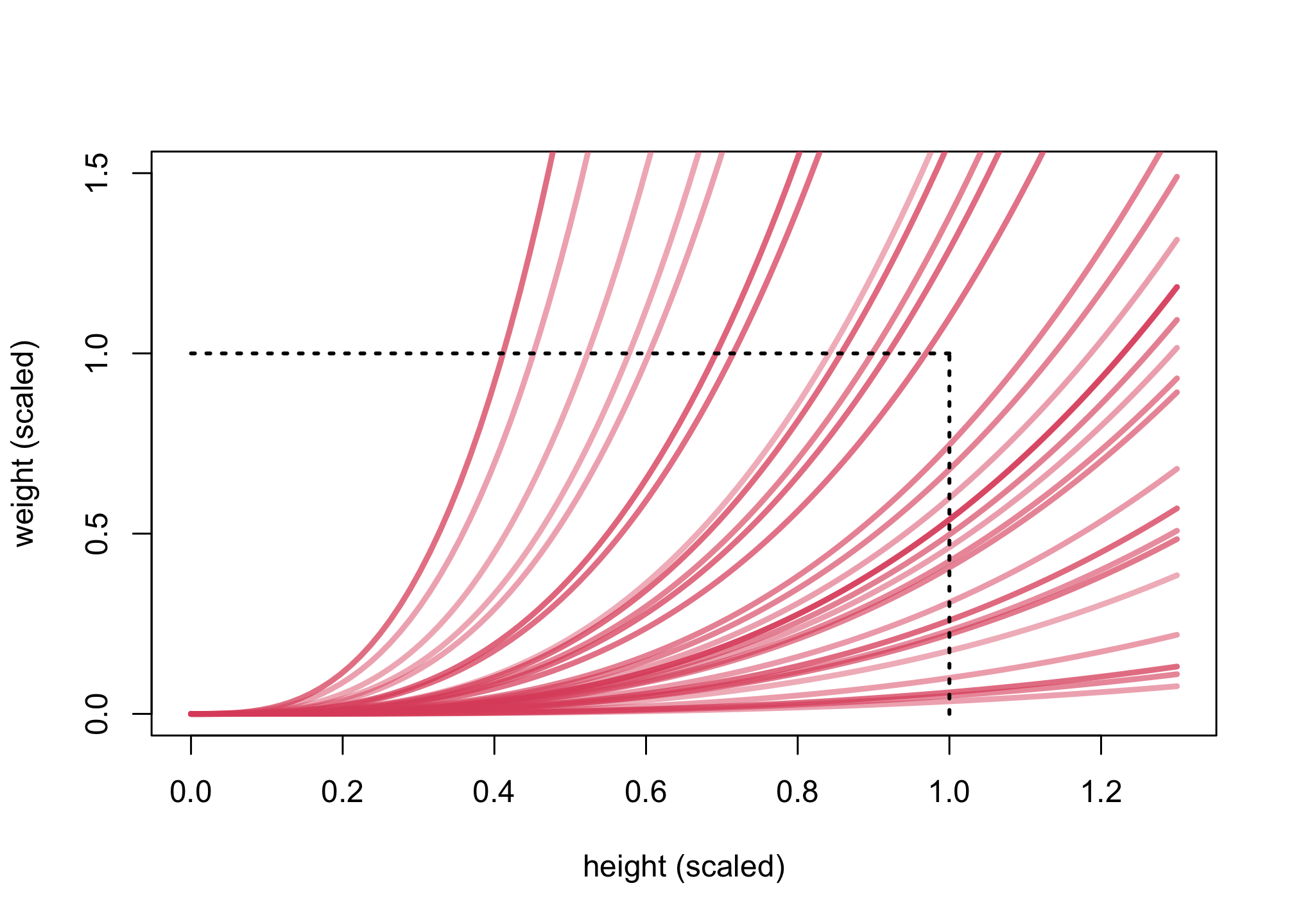
Prior Predictive Check
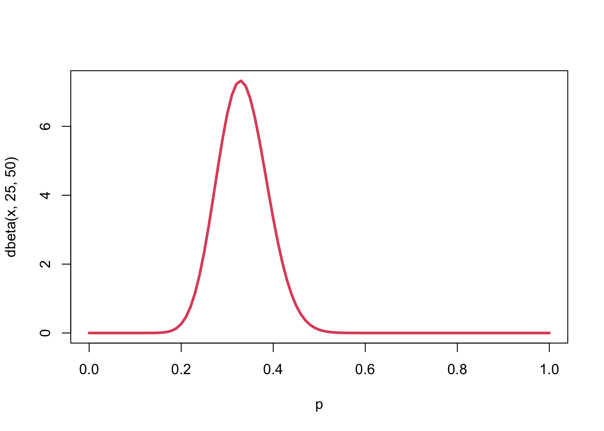
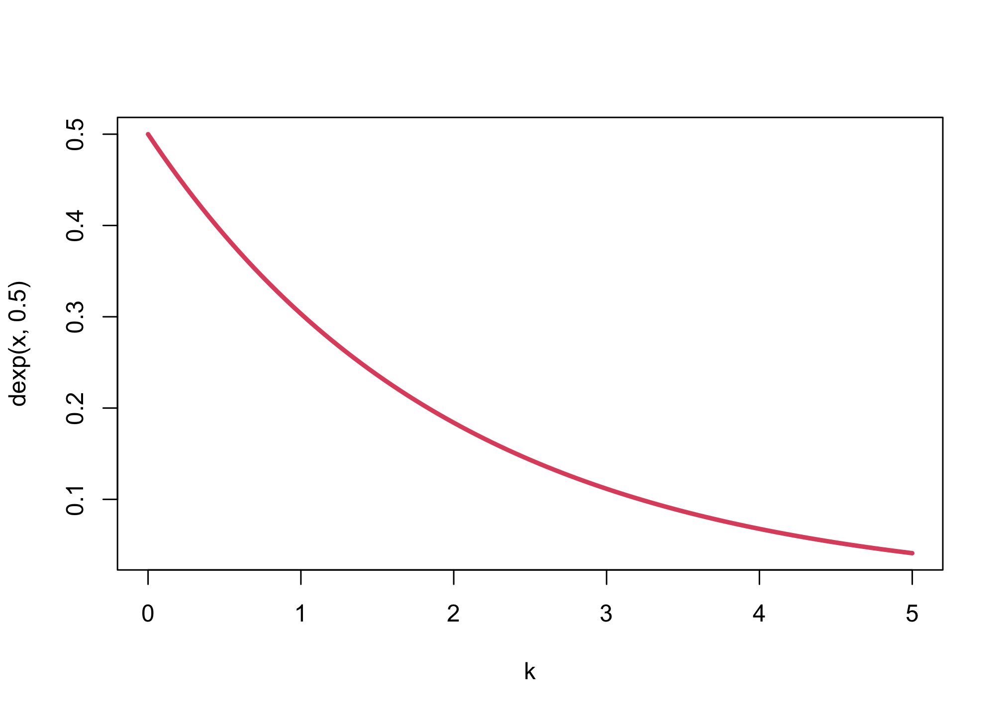
The key will be to select the priors for \(k\) and \(p\). We’ll select \(p \sim Beta(25,50)\) given that this would imply the prior will have a mean of \(25 / (25 + 50) = 1/3\), given we’re selecting a \(Beta\) distribution. For \(k\), we’ll use \(Exponential(0.5)\) given that this value represents the kilograms per cubic centimeters. Note that the priors shown in Lecture 19 are slightly different than what’s in the textbook. We’ll use Lecture 19 values.
n <- 30
p <- rbeta(1e4,25,50)
k <- rexp(1e4,0.5)
sigma <- rexp(n,1)
xseq <- seq(from=0,to=1.3,len=100)
plot(NULL,xlim=c(0,1.3),ylim=c(0,1.5),xlab="height (scaled)",ylab="weight (scaled)")
for ( i in 1:n ) {
    mu <- log( pi * k[i] * p[i]^2 * xseq^3 )
    lines( xseq , exp(mu + sigma[i]^2/2) , lwd=3 , col=col.alpha(2,runif(1,0.4,0.8)) )
}
lines( c(1,1) , c(0,1) , lty=3 , lwd=2 )
lines( c(0,1) , c(1,1) , lty=3 , lwd=2 )
curve( dbeta(x,25,50) , from=0, to=1 , xlim=c(0,1) , lwd=3 , col=2 , xlab="p")
curve( dexp(x,0.5) , from=0, to=5 , xlim=c(0,5) , lwd=3 , col=2 , xlab="k")
Initial Model
Given our statistical model above, let’s write out our model:
dat <- list(W=d$w,H=d$h)
m16.1 <- ulam(
    alist(
        W ~ dlnorm( mu , sigma ),
        exp(mu) <- 3.141593 * k * p^2 * H^3,
        p ~ beta( 25 , 50 ),
        k ~ exponential( 0.5 ),
        sigma ~ exponential( 1 )
    ), data=dat , chains=4 , cores=4 )
## Running MCMC with 4 parallel chains, with 1 thread(s) per chain...
##
## Chain 1 Iteration:   1 / 1000 [  0%]  (Warmup)
## Chain 2 Iteration:   1 / 1000 [  0%]  (Warmup)
## Chain 2 Iteration: 100 / 1000 [ 10%]  (Warmup)
## Chain 3 Iteration:   1 / 1000 [  0%]  (Warmup)
## Chain 4 Iteration:   1 / 1000 [  0%]  (Warmup)
## Chain 3 Iteration: 100 / 1000 [ 10%]  (Warmup)
## Chain 4 Iteration: 100 / 1000 [ 10%]  (Warmup)
## Chain 1 Iteration: 100 / 1000 [ 10%]  (Warmup)
## Chain 2 Iteration: 200 / 1000 [ 20%]  (Warmup)
## Chain 3 Iteration: 200 / 1000 [ 20%]  (Warmup)
## Chain 1 Iteration: 200 / 1000 [ 20%]  (Warmup)
## Chain 4 Iteration: 200 / 1000 [ 20%]  (Warmup)
## Chain 3 Iteration: 300 / 1000 [ 30%]  (Warmup)
## Chain 1 Iteration: 300 / 1000 [ 30%]  (Warmup)
## Chain 2 Iteration: 300 / 1000 [ 30%]  (Warmup)
## Chain 4 Iteration: 300 / 1000 [ 30%]  (Warmup)
## Chain 3 Iteration: 400 / 1000 [ 40%]  (Warmup)
## Chain 1 Iteration: 400 / 1000 [ 40%]  (Warmup)
## Chain 4 Iteration: 400 / 1000 [ 40%]  (Warmup)
## Chain 2 Iteration: 400 / 1000 [ 40%]  (Warmup)
## Chain 3 Iteration: 500 / 1000 [ 50%]  (Warmup)
## Chain 3 Iteration: 501 / 1000 [ 50%]  (Sampling)
## Chain 4 Iteration: 500 / 1000 [ 50%]  (Warmup)
## Chain 4 Iteration: 501 / 1000 [ 50%]  (Sampling)
## Chain 1 Iteration: 500 / 1000 [ 50%]  (Warmup)
## Chain 1 Iteration: 501 / 1000 [ 50%]  (Sampling)
## Chain 2 Iteration: 500 / 1000 [ 50%]  (Warmup)
## Chain 2 Iteration: 501 / 1000 [ 50%]  (Sampling)
## Chain 3 Iteration: 600 / 1000 [ 60%]  (Sampling)
## Chain 1 Iteration: 600 / 1000 [ 60%]  (Sampling)
## Chain 2 Iteration: 600 / 1000 [ 60%]  (Sampling)
## Chain 4 Iteration: 600 / 1000 [ 60%]  (Sampling)
## Chain 3 Iteration: 700 / 1000 [ 70%]  (Sampling)
## Chain 1 Iteration: 700 / 1000 [ 70%]  (Sampling)
## Chain 2 Iteration: 700 / 1000 [ 70%]  (Sampling)
## Chain 4 Iteration: 700 / 1000 [ 70%]  (Sampling)
## Chain 3 Iteration: 800 / 1000 [ 80%]  (Sampling)
## Chain 1 Iteration: 800 / 1000 [ 80%]  (Sampling)
## Chain 2 Iteration: 800 / 1000 [ 80%]  (Sampling)
## Chain 4 Iteration: 800 / 1000 [ 80%]  (Sampling)
## Chain 3 Iteration: 900 / 1000 [ 90%]  (Sampling)
## Chain 1 Iteration: 900 / 1000 [ 90%]  (Sampling)
## Chain 2 Iteration: 900 / 1000 [ 90%]  (Sampling)
## Chain 4 Iteration: 900 / 1000 [ 90%]  (Sampling)
## Chain 3 Iteration: 1000 / 1000 [100%]  (Sampling)
## Chain 3 finished in 5.4 seconds.
## Chain 1 Iteration: 1000 / 1000 [100%]  (Sampling)
## Chain 2 Iteration: 1000 / 1000 [100%]  (Sampling)
## Chain 1 finished in 5.4 seconds.
## Chain 2 finished in 5.4 seconds.
## Chain 4 Iteration: 1000 / 1000 [100%]  (Sampling)
## Chain 4 finished in 5.6 seconds.
##
## All 4 chains finished successfully.
## Mean chain execution time: 5.5 seconds.
## Total execution time: 5.8 seconds.
Fit Model
precis(m16.1)
##            mean          sd      5.5%     94.5%    n_eff     Rhat4
## p     0.3443633 0.051311427 0.2656361 0.4307825 447.2716 1.0092353
## k     2.7222224 0.842208350 1.6298986 4.2651270 464.2493 1.0088055
## sigma 0.2069968 0.006046353 0.1977088 0.2169148 849.0182 0.9995161
Convergence
traceplot(m16.1)
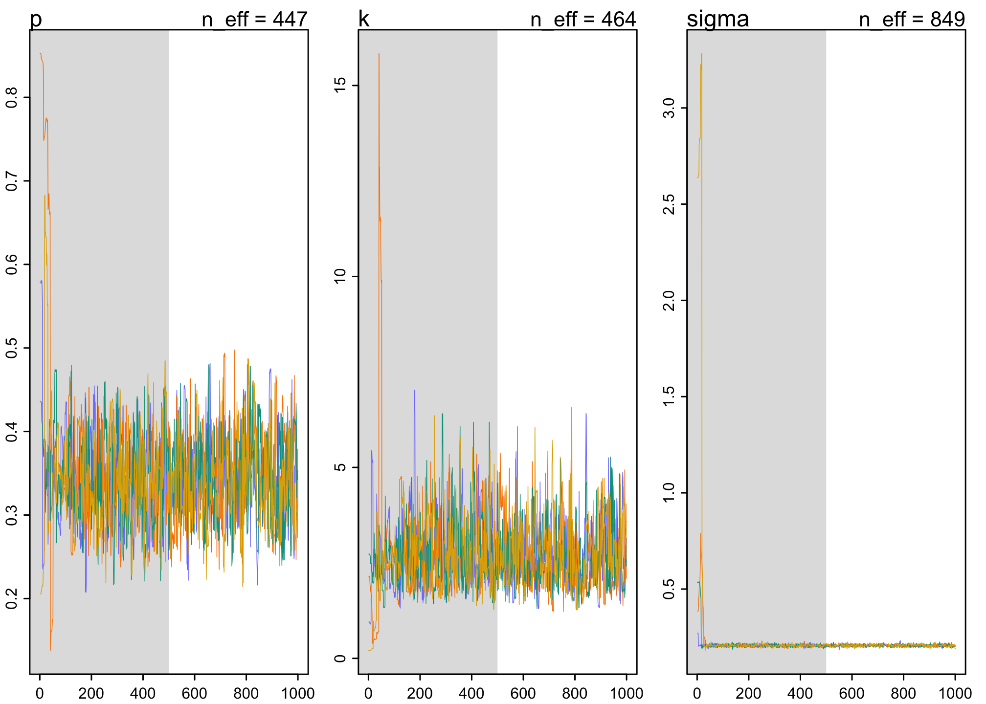
We find sufficient model convergence in the traceplots, consistent with the Rhat.
Posterior Predictive Simulation
Let’s do a posterior predictive simulation.
h_seq <- seq( from=0 , to=max(d$h) , length.out=100 )
w_sim <- sim( m16.1 , data=list(H=h_seq) )
mu_mean <- apply( w_sim , 2 , mean )
w_CI <- apply( w_sim , 2 , PI )
plot( d$h , d$w , xlim=c(0,max(d$h)) , ylim=c(0,max(d$w)) , col=2 ,
    lwd=2 , xlab="height (scaled)" , ylab="weight (scaled)" )
shade( w_CI , h_seq , col=col.alpha(2,0.5) )
lines( h_seq , mu_mean , lwd=3 )
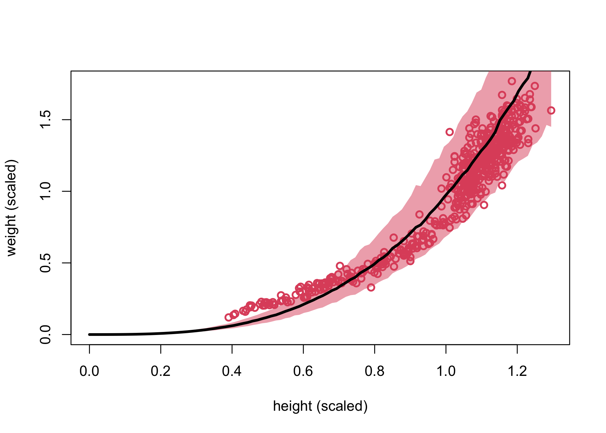
We can see that with the exception of children (i.e., small weight/height), the cylinder model does a fairly good job of fitting the model. You can review Lecture 19 for more details on how we can rewrite different versions of this model.
Population Dynamics
Let’s also review the Lynx and Hare example in Lecture 19 and Chapter 16.
## R code 16.13
library(rethinking)
data(Lynx_Hare)
Lynx_Hare
##    Year Lynx Hare
## 1  1900  4.0 30.0
## 2  1901  6.1 47.2
## 3  1902  9.8 70.2
## 4  1903 35.2 77.4
## 5  1904 59.4 36.3
## 6  1905 41.7 20.6
## 7  1906 19.0 18.1
## 8  1907 13.0 21.4
## 9  1908  8.3 22.0
## 10 1909  9.1 25.4
## 11 1910  7.4 27.1
## 12 1911  8.0 40.3
## 13 1912 12.3 57.0
## 14 1913 19.5 76.6
## 15 1914 45.7 52.3
## 16 1915 51.1 19.5
## 17 1916 29.7 11.2
## 18 1917 15.8  7.6
## 19 1918  9.7 14.6
## 20 1919 10.1 16.2
## 21 1920  8.6 24.7
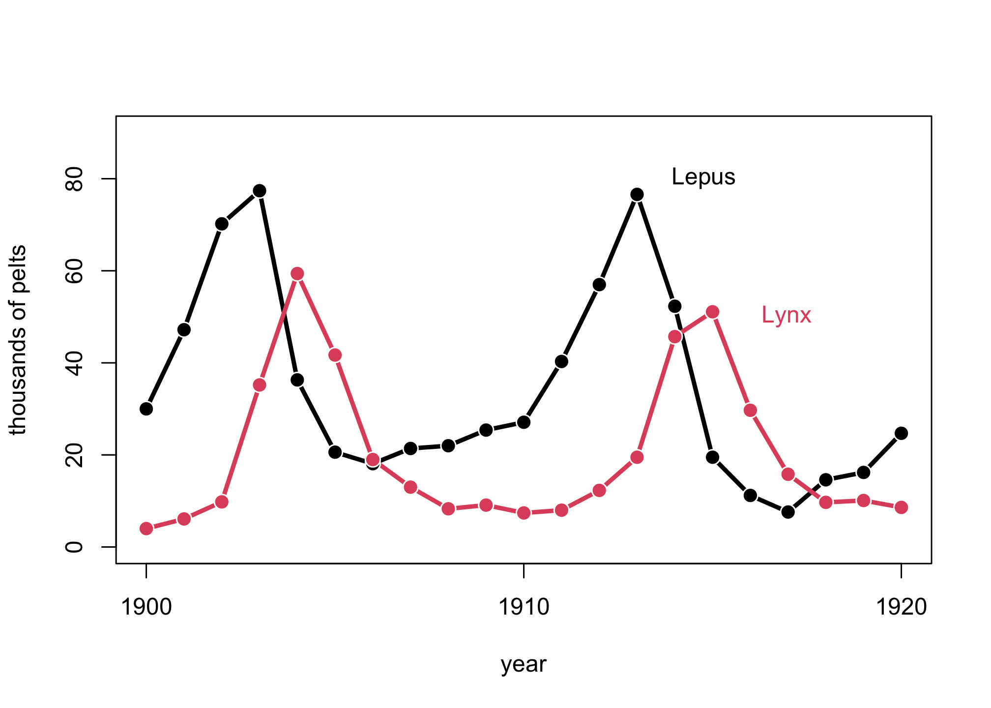
Let’s plot the data.
plot( 1:21 , Lynx_Hare[,3] , ylim=c(0,90) , xlab="year" ,
    ylab="thousands of pelts" , xaxt="n" , type="l" , lwd=3  )
at <- c(1,11,21)
axis( 1 , at=at , labels=Lynx_Hare$Year[at] )
lines( 1:21 , Lynx_Hare[,2] , lwd=3 , col=2 )
points( 1:21 , Lynx_Hare[,3] , bg="black" , col="white" , pch=21 , cex=1.4 )
points( 1:21 , Lynx_Hare[,2] , bg=2 , col="white" , pch=21 , cex=1.4 )
text( 17 , 80 , "Lepus" , pos=2 )
text( 19 , 50 , "Lynx" , pos=2 , col=2 )
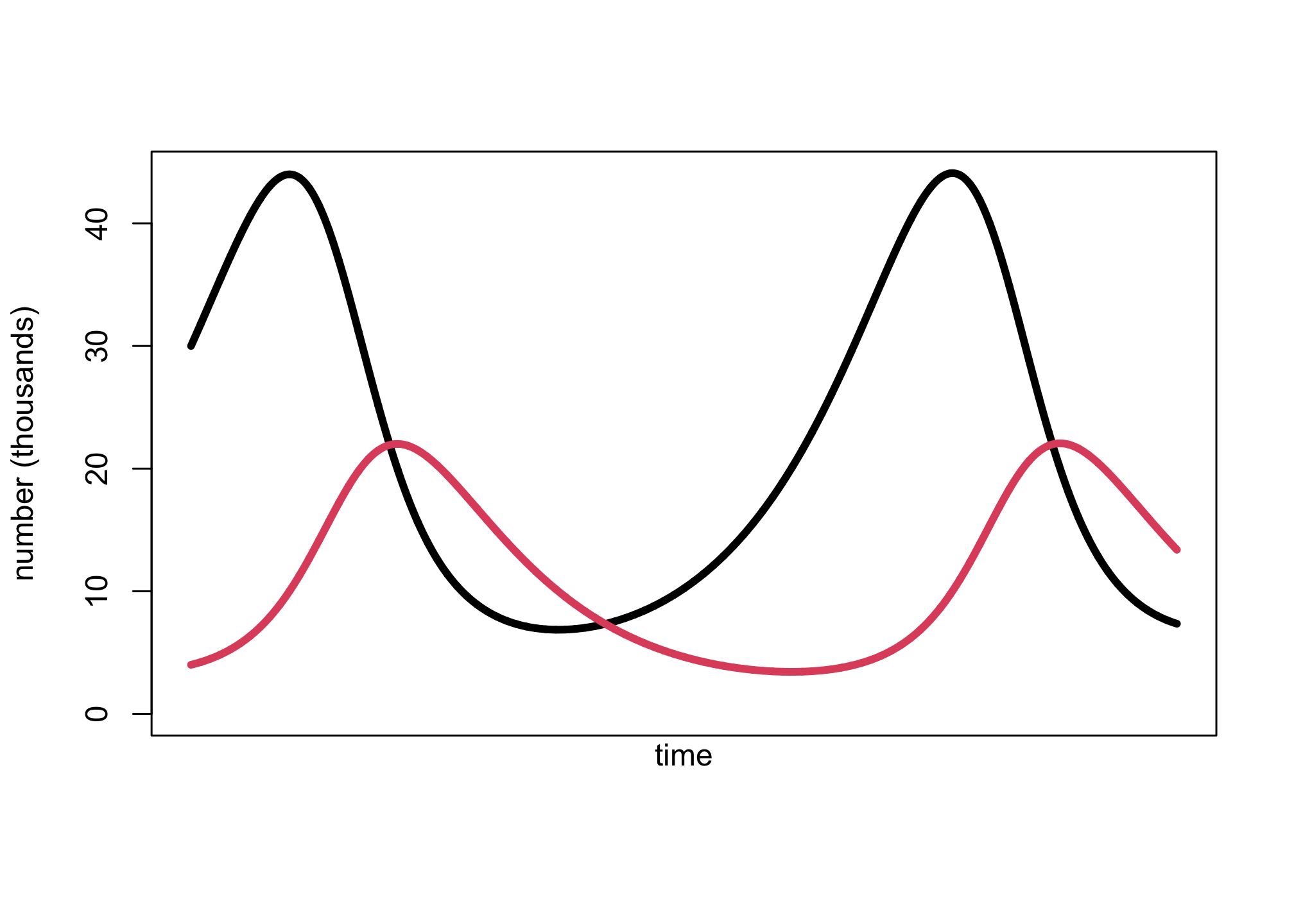
Generative Model
Let’s create a generative model. This is based on the ordinary differential equations laid out in Lecture 19. See Lecture 19 for the intuition around the equations.
## R code 16.14
sim_lynx_hare <- function( n_steps , init , theta , dt=0.002 ) {
    L <- rep(NA,n_steps)
    H <- rep(NA,n_steps)
    L[1] <- init[1]
    H[1] <- init[2]
    for ( i in 2:n_steps ) {
        H[i] <- H[i-1] + dt*H[i-1]*( theta[1] - theta[2]*L[i-1] )
        L[i] <- L[i-1] + dt*L[i-1]*( theta[3]*H[i-1] - theta[4] )
    }
    return( cbind(L,H) )
}

## R code 16.15
theta <- c( 0.5 , 0.05 , 0.025 , 0.5 )
z <- sim_lynx_hare( 1e4 , as.numeric(Lynx_Hare[1,2:3]) , theta )

plot( z[,2] , type="l" , ylim=c(0,max(z[,2])) , lwd=4 , xaxt="n" ,
    ylab="number (thousands)" , xlab="" )
lines( z[,1] , col=2 , lwd=4 )
mtext( "time" , 1 )
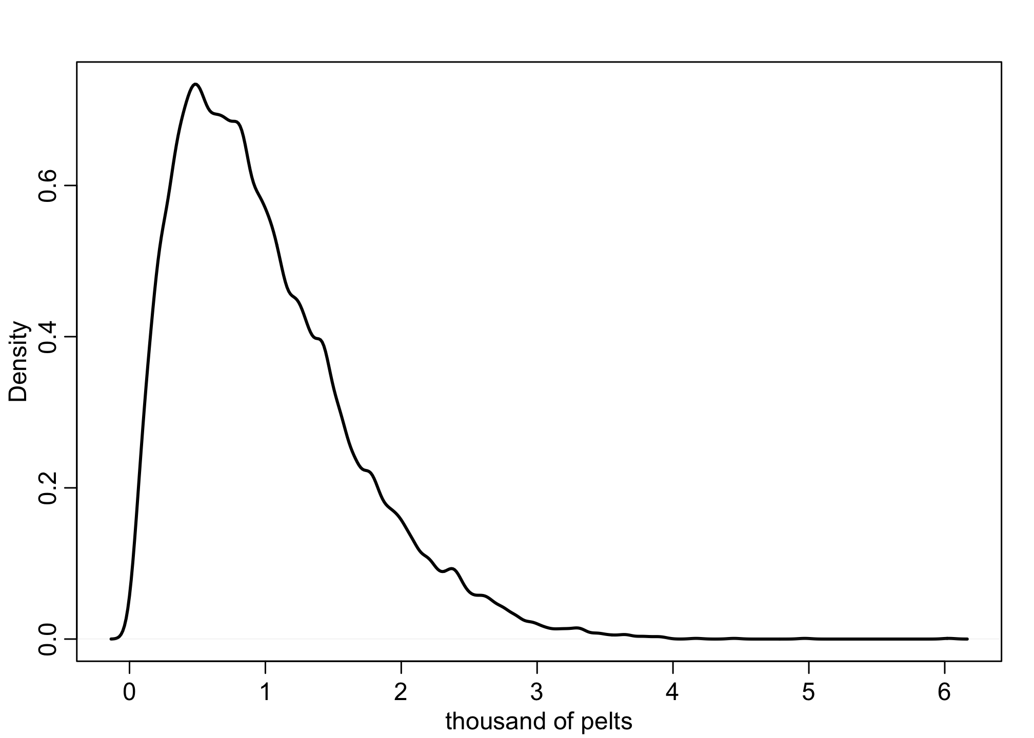
Prior Predictive Simulation
## R code 16.16
N <- 1e4
Ht <- 1e4
p <- rbeta(N,2,18)
h <- rbinom( N , size=Ht , prob=p )
h <- round( h/1000 , 2 )
dens( h , xlab="thousand of pelts" , lwd=2 )
Initial Model
Let’s specify our model.
## R code 16.17
data(Lynx_Hare_model)
cat(Lynx_Hare_model) # Stan model specifications (see Lecture 19)
## functions {
##   real[] dpop_dt( real t,                 // time
##                 real[] pop_init,          // initial state {lynx, hares}
##                 real[] theta,             // parameters
##                 real[] x_r, int[] x_i) {  // unused
##     real L = pop_init[1];
##     real H = pop_init[2];
##     real bh = theta[1];
##     real mh = theta[2];
##     real ml = theta[3];
##     real bl = theta[4];
##     // differential equations
##     real dH_dt = (bh - mh * L) * H;
##     real dL_dt = (bl * H - ml) * L;
##     return { dL_dt , dH_dt };
##   }
## }
## data {
##   int<lower=0> N;              // number of measurement times
##   real<lower=0> pelts[N,2];    // measured populations
## }
## transformed data{
##   real times_measured[N-1];    // N-1 because first time is initial state
##   for ( i in 2:N ) times_measured[i-1] = i;
## }
## parameters {
##   real<lower=0> theta[4];      // { bh, mh, ml, bl }
##   real<lower=0> pop_init[2];   // initial population state
##   real<lower=0> sigma[2];      // measurement errors
##   real<lower=0,upper=1> p[2];  // trap rate
## }
## transformed parameters {
##   real pop[N, 2];
##   pop[1,1] = pop_init[1];
##   pop[1,2] = pop_init[2];
##   pop[2:N,1:2] = integrate_ode_rk45(
##     dpop_dt, pop_init, 0, times_measured, theta,
##     rep_array(0.0, 0), rep_array(0, 0),
##     1e-5, 1e-3, 5e2);
## }
## model {
##   // priors
##   theta[{1,3}] ~ normal( 1 , 0.5 );    // bh,ml
##   theta[{2,4}] ~ normal( 0.05, 0.05 ); // mh,bl
##   sigma ~ exponential( 1 );
##   pop_init ~ lognormal( log(10) , 1 );
##   p ~ beta(40,200);
##   // observation model
##   // connect latent population state to observed pelts
##   for ( t in 1:N )
##     for ( k in 1:2 )
##       pelts[t,k] ~ lognormal( log(pop[t,k]*p[k]) , sigma[k] );
## }
## generated quantities {
##   real pelts_pred[N,2];
##   for ( t in 1:N )
##     for ( k in 1:2 )
##       pelts_pred[t,k] = lognormal_rng( log(pop[t,k]*p[k]) , sigma[k] );
## }
We can now run the model into cstan.
## R code 16.18
dat_list <- list(
    N = nrow(Lynx_Hare),
    pelts = Lynx_Hare[,2:3] )

m16.5 <- cstan( model_code=Lynx_Hare_model , data=dat_list , chains=3 ,
    cores=3 , control=list( adapt_delta=0.95 ) )
## Running MCMC with 3 parallel chains...
##
## Chain 1 Iteration:   1 / 1000 [  0%]  (Warmup)
## Chain 2 Iteration:   1 / 1000 [  0%]  (Warmup)
## Chain 3 Iteration:   1 / 1000 [  0%]  (Warmup)
## Chain 1 Iteration: 100 / 1000 [ 10%]  (Warmup)
## Chain 3 Iteration: 100 / 1000 [ 10%]  (Warmup)
## Chain 1 Iteration: 200 / 1000 [ 20%]  (Warmup)
## Chain 2 Iteration: 100 / 1000 [ 10%]  (Warmup)
## Chain 3 Iteration: 200 / 1000 [ 20%]  (Warmup)
## Chain 1 Iteration: 300 / 1000 [ 30%]  (Warmup)
## Chain 2 Iteration: 200 / 1000 [ 20%]  (Warmup)
## Chain 1 Iteration: 400 / 1000 [ 40%]  (Warmup)
## Chain 3 Iteration: 300 / 1000 [ 30%]  (Warmup)
## Chain 2 Iteration: 300 / 1000 [ 30%]  (Warmup)
## Chain 1 Iteration: 500 / 1000 [ 50%]  (Warmup)
## Chain 1 Iteration: 501 / 1000 [ 50%]  (Sampling)
## Chain 3 Iteration: 400 / 1000 [ 40%]  (Warmup)
## Chain 1 Iteration: 600 / 1000 [ 60%]  (Sampling)
## Chain 2 Iteration: 400 / 1000 [ 40%]  (Warmup)
## Chain 3 Iteration: 500 / 1000 [ 50%]  (Warmup)
## Chain 3 Iteration: 501 / 1000 [ 50%]  (Sampling)
## Chain 1 Iteration: 700 / 1000 [ 70%]  (Sampling)
## Chain 2 Iteration: 500 / 1000 [ 50%]  (Warmup)
## Chain 2 Iteration: 501 / 1000 [ 50%]  (Sampling)
## Chain 1 Iteration: 800 / 1000 [ 80%]  (Sampling)
## Chain 3 Iteration: 600 / 1000 [ 60%]  (Sampling)
## Chain 1 Iteration: 900 / 1000 [ 90%]  (Sampling)
## Chain 2 Iteration: 600 / 1000 [ 60%]  (Sampling)
## Chain 3 Iteration: 700 / 1000 [ 70%]  (Sampling)
## Chain 1 Iteration: 1000 / 1000 [100%]  (Sampling)
## Chain 1 finished in 8.1 seconds.
## Chain 3 Iteration: 800 / 1000 [ 80%]  (Sampling)
## Chain 2 Iteration: 700 / 1000 [ 70%]  (Sampling)
## Chain 3 Iteration: 900 / 1000 [ 90%]  (Sampling)
## Chain 2 Iteration: 800 / 1000 [ 80%]  (Sampling)
## Chain 3 Iteration: 1000 / 1000 [100%]  (Sampling)
## Chain 3 finished in 10.3 seconds.
## Chain 2 Iteration: 900 / 1000 [ 90%]  (Sampling)
## Chain 2 Iteration: 1000 / 1000 [100%]  (Sampling)
## Chain 2 finished in 12.0 seconds.
##
## All 3 chains finished successfully.
## Mean chain execution time: 10.2 seconds.
## Total execution time: 12.2 seconds.
precis(m16.5, depth=2)
##                     mean           sd         5.5%        94.5%     n_eff
## theta[1]    5.259743e-01 5.930876e-02 4.363824e-01 6.260182e-01  783.8612
## theta[2]    4.696245e-03 9.733230e-04 3.254495e-03 6.357309e-03  759.0839
## theta[3]    8.163002e-01 9.126050e-02 6.807107e-01 9.648221e-01  766.4677
## theta[4]    4.353289e-03 8.730685e-04 3.039033e-03 5.796600e-03  742.8976
## pop_init[1] 3.649332e+01 6.578326e+00 2.698149e+01 4.770728e+01  772.9639
## pop_init[2] 1.425877e+02 2.415005e+01 1.097513e+02 1.826711e+02  858.3767
## sigma[1]    2.638355e-01 4.742685e-02 1.977493e-01 3.476656e-01 1179.1647
## sigma[2]    2.499734e-01 4.270254e-02 1.937928e-01 3.288712e-01 1133.8828
## p[1]        1.745459e-01 2.502233e-02 1.364659e-01 2.157365e-01  759.9731
## p[2]        1.791307e-01 2.441394e-02 1.404702e-01 2.177944e-01  905.6766
##                 Rhat4
## theta[1]    1.0006137
## theta[2]    1.0027718
## theta[3]    1.0001022
## theta[4]    1.0029659
## pop_init[1] 1.0016562
## pop_init[2] 1.0013906
## sigma[1]    0.9993528
## sigma[2]    1.0012667
## p[1]        1.0004058
## p[2]        1.0020569
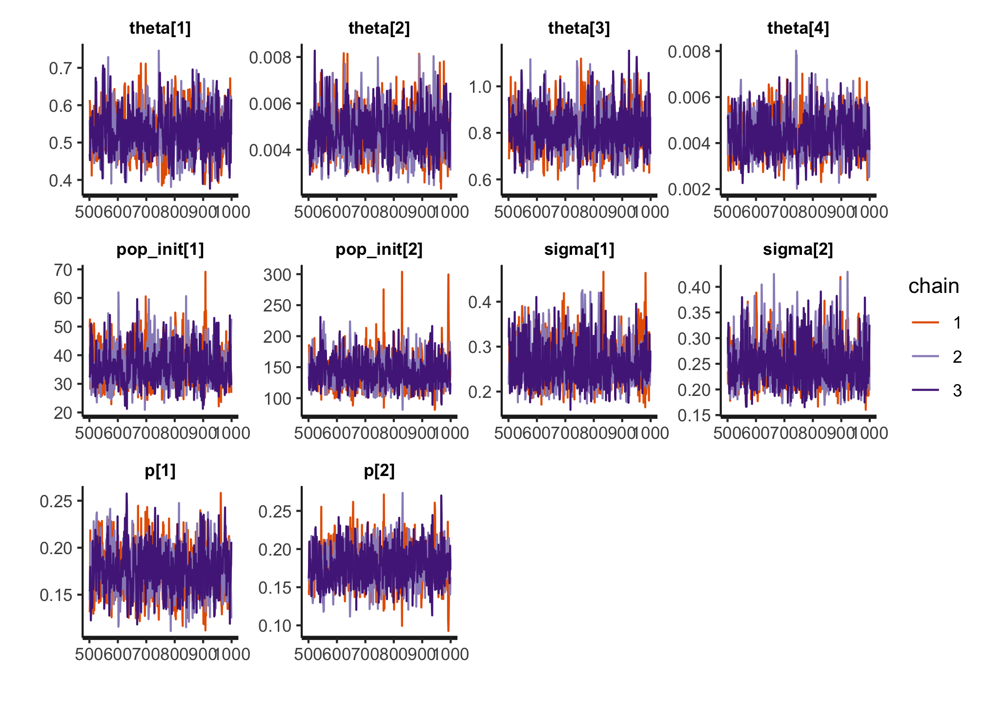
Convergence
traceplot(m16.5)
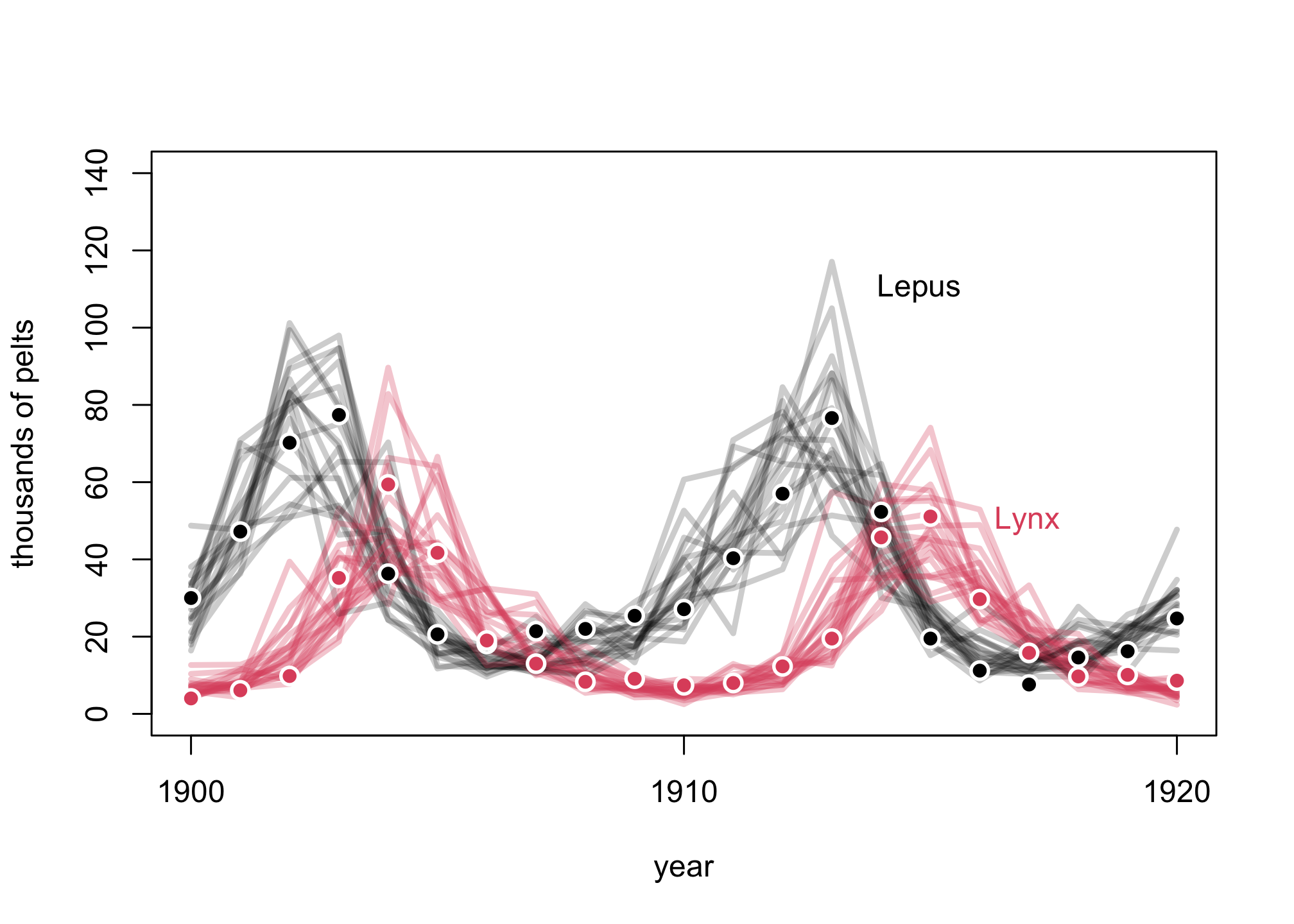
Posterior Predictive Simulation
## R code 16.19
post <- extract.samples(m16.5)
pelts <- dat_list$pelts
plot( 1:21 , pelts[,2] , pch=16 , ylim=c(0,140) , xlab="year" ,
    ylab="thousands of pelts" , xaxt="n" )
at <- c(1,11,21)
axis( 1 , at=at , labels=Lynx_Hare$Year[at] )
# 21 time series from posterior
for ( s in 1:21 ) {
    lines( 1:21 , post$pelts_pred[s,,2] , col=col.alpha("black",0.2) , lwd=3 )
    lines( 1:21 , post$pelts_pred[s,,1] , col=col.alpha(2,0.3) , lwd=3 )
}
# points
points( 1:21 , pelts[,2] , col="white" , pch=16 , cex=1.5 )
points( 1:21 , pelts[,2] , col=1 , pch=16 )
points( 1:21 , pelts[,1] , col="white" , pch=16 , cex=1.5 )
points( 1:21 , pelts[,1] , col=2 , pch=16 )
# text labels
text( 17 , 110 , "Lepus" , pos=2 )
text( 19 , 50 , "Lynx" , pos=2 , col=2 )
Package versions
sessionInfo()
## R version 4.1.1 (2021-08-10)
## Platform: aarch64-apple-darwin20 (64-bit)
## Running under: macOS Monterey 12.3.1
##
## Matrix products: default
## BLAS:   /Library/Frameworks/R.framework/Versions/4.1-arm64/Resources/lib/libRblas.0.dylib
## LAPACK: /Library/Frameworks/R.framework/Versions/4.1-arm64/Resources/lib/libRlapack.dylib
##
## locale:
## [1] en_US.UTF-8/en_US.UTF-8/en_US.UTF-8/C/en_US.UTF-8/en_US.UTF-8
##
## attached base packages:
## [1] parallel  stats     graphics  grDevices datasets  utils     methods
## [8] base
##
## other attached packages:
## [1] digest_0.6.29        rethinking_2.21      cmdstanr_0.4.0.9001
## [4] rstan_2.21.3         ggplot2_3.3.5        StanHeaders_2.21.0-7
##
## loaded via a namespace (and not attached):
##  [1] sass_0.4.0           jsonlite_1.7.2       bslib_0.3.1
##  [4] RcppParallel_5.1.4   assertthat_0.2.1     posterior_1.1.0
##  [7] distributional_0.2.2 highr_0.9            stats4_4.1.1
## [10] tensorA_0.36.2       renv_0.14.0          yaml_2.2.1
## [13] pillar_1.6.4         backports_1.4.1      lattice_0.20-44
## [16] glue_1.6.0           checkmate_2.0.0      colorspace_2.0-2
## [19] htmltools_0.5.2      pkgconfig_2.0.3      bookdown_0.24
## [22] purrr_0.3.4          mvtnorm_1.1-3        scales_1.1.1
## [25] processx_3.5.2       tibble_3.1.6         generics_0.1.1
## [28] farver_2.1.0         ellipsis_0.3.2       withr_2.4.3
## [31] cli_3.1.0            magrittr_2.0.1       crayon_1.4.2
## [34] mime_0.12            evaluate_0.14        ps_1.6.0
## [37] fs_1.5.0             fansi_0.5.0          MASS_7.3-54
## [40] pkgbuild_1.3.1       blogdown_1.5         tools_4.1.1
## [43] loo_2.4.1            data.table_1.14.2    prettyunits_1.1.1
## [46] lifecycle_1.0.1      matrixStats_0.61.0   stringr_1.4.0
## [49] munsell_0.5.0        callr_3.7.0          compiler_4.1.1
## [52] jquerylib_0.1.4      rlang_0.4.12         grid_4.1.1
## [55] rstudioapi_0.13      labeling_0.4.2       base64enc_0.1-3
## [58] rmarkdown_2.11       gtable_0.3.0         codetools_0.2-18
## [61] inline_0.3.19        abind_1.4-5          DBI_1.1.1
## [64] R6_2.5.1             gridExtra_2.3        lubridate_1.8.0
## [67] knitr_1.36           dplyr_1.0.7          fastmap_1.1.0
## [70] utf8_1.2.2           downloadthis_0.2.1   bsplus_0.1.3
## [73] shape_1.4.6          stringi_1.7.6        Rcpp_1.0.7
## [76] vctrs_0.3.8          tidyselect_1.1.1     xfun_0.28
## [79] coda_0.19-4