Class 7
In-Class Lab
Rethinking: Section 7.5.1
library(rethinking)

## R code 6.13
set.seed(71)
# number of plants
N <- 100

# simulate initial heights
h0 <- rnorm(N,10,2)

# assign treatments and simulate fungus and growth
treatment <- rep( 0:1 , each=N/2 )
fungus <- rbinom( N , size=1 , prob=0.5 - treatment*0.4 )
h1 <- h0 + rnorm(N, 5 - 3*fungus)

# compose a clean data frame
d <- data.frame( h0=h0 , h1=h1 , treatment=treatment , fungus=fungus )
precis(d)
##               mean        sd      5.5%    94.5%    histogram
## h0         9.95978 2.1011623  6.570328 13.07874 ▁▂▂▂▇▃▂▃▁▁▁▁
## h1        14.39920 2.6880870 10.618002 17.93369     ▁▁▃▇▇▇▁▁
## treatment  0.50000 0.5025189  0.000000  1.00000   ▇▁▁▁▁▁▁▁▁▇
## fungus     0.23000 0.4229526  0.000000  1.00000   ▇▁▁▁▁▁▁▁▁▂
## R code 6.14
sim_p <- rlnorm( 1e4 , 0 , 0.25 )
precis( data.frame(sim_p) )
##          mean        sd     5.5%    94.5%    histogram
## sim_p 1.03699 0.2629894 0.670683 1.496397 ▁▁▃▇▇▃▁▁▁▁▁▁
Recall:
m6.6 = model with just an intercept
m6.7 = model includes treatment and fungus (post-treatment bias)
m6.8 = model with just treatment and correctly infers causal influence of the treatment
## R code 6.15
m6.6 <- quap(
  alist(
    h1 ~ dnorm( mu , sigma ),
    mu <- h0*p,
    p ~ dlnorm( 0 , 0.25 ),
    sigma ~ dexp( 1 )
  ), data=d )
precis(m6.6)
##           mean         sd     5.5%    94.5%
## p     1.426626 0.01760992 1.398482 1.454770
## sigma 1.793286 0.12517262 1.593236 1.993336
## R code 6.16
m6.7 <- quap(
  alist(
    h1 ~ dnorm( mu , sigma ),
    mu <- h0 * p,
    p <- a + bt*treatment + bf*fungus,
    a ~ dlnorm( 0 , 0.2 ) ,
    bt ~ dnorm( 0 , 0.5 ),
    bf ~ dnorm( 0 , 0.5 ),
    sigma ~ dexp( 1 )
  ), data=d )
precis(m6.7)
##               mean         sd        5.5%       94.5%
## a      1.481391468 0.02451069  1.44221865  1.52056429
## bt     0.002412222 0.02986965 -0.04532525  0.05014969
## bf    -0.266718915 0.03654772 -0.32512923 -0.20830860
## sigma  1.408797442 0.09862070  1.25118251  1.56641237
## R code 6.17
m6.8 <- quap(
  alist(
    h1 ~ dnorm( mu , sigma ),
    mu <- h0 * p,
    p <- a + bt*treatment,
    a ~ dlnorm( 0 , 0.2 ),
    bt ~ dnorm( 0 , 0.5 ),
    sigma ~ dexp( 1 )
  ), data=d )
precis(m6.8)
##             mean         sd       5.5%     94.5%
## a     1.38035767 0.02517554 1.34012229 1.4205931
## bt    0.08499924 0.03429718 0.03018573 0.1398128
## sigma 1.74631655 0.12191552 1.55147200 1.9411611
# 7.25
set.seed(11)
WAIC(m6.7)
##       WAIC      lppd  penalty  std_err
## 1 361.4511 -177.1724 3.553198 14.17033
set.seed(77)
compare(m6.6, m6.7, m6.8, func=WAIC)
##          WAIC       SE    dWAIC      dSE    pWAIC       weight
## m6.7 361.8901 14.26190  0.00000       NA 3.839491 1.000000e+00
## m6.8 402.7757 11.28257 40.88562 10.47837 2.645879 1.323732e-09
## m6.6 405.9139 11.64641 44.02380 12.22582 1.581312 2.756471e-10
WAIC = smaller values are better and the models are ordered by WAIC, best to worst.
pWAIC = penalty term of WAIC.
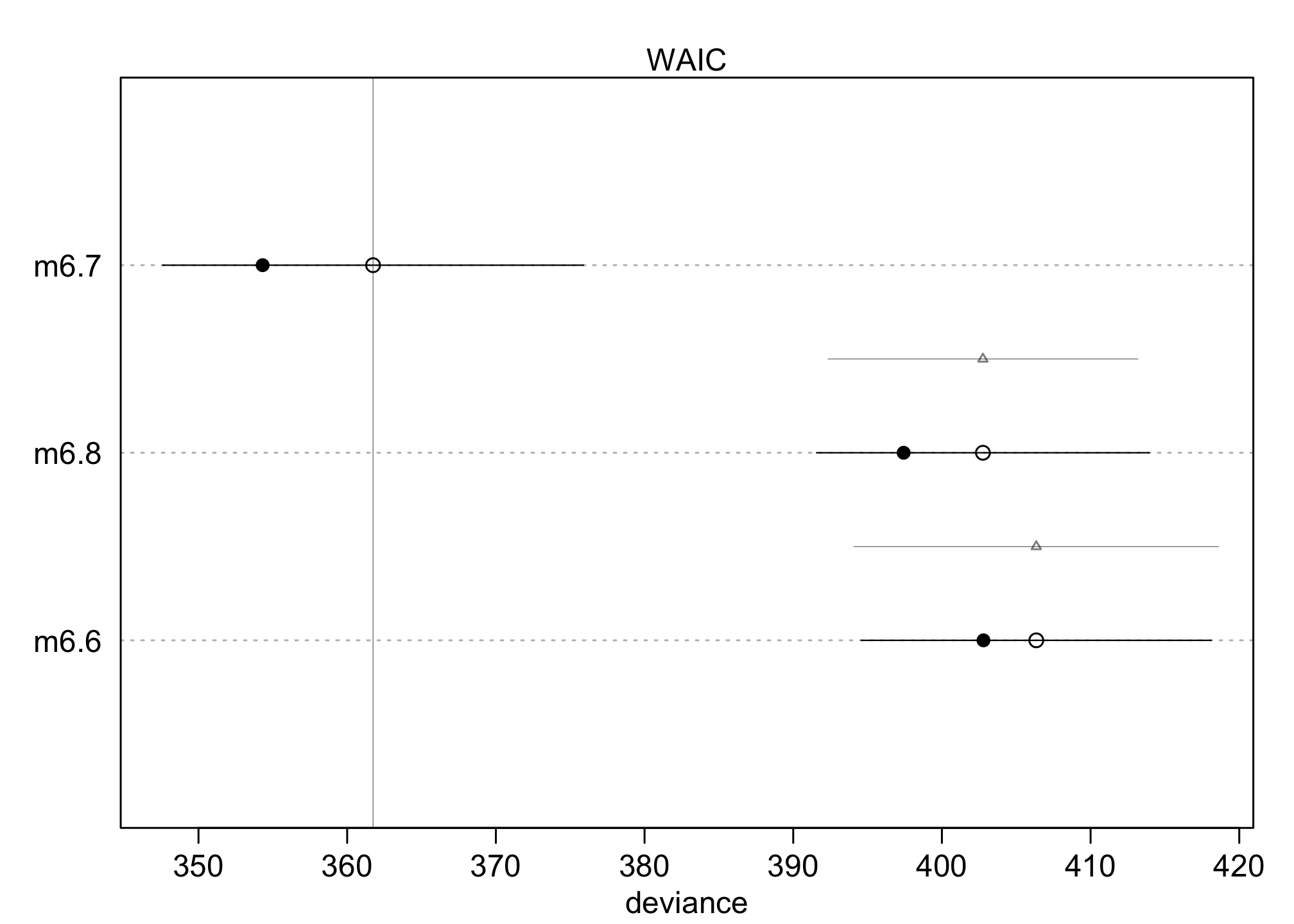
plot(compare(m6.6, m6.7, m6.8))

The filled points are the in-sample deviance values. The open points are the WAIC values. Notice that naturally each model does better in-sample than it is expected to do out-of-sample. The line segments show the standard error of each WAIC. These are the values in the column labeled SE in the table above.
So you can probably see how much better m6.7 is than m6.8. What we really want however is the standard error of the difference in WAIC between the two models. That is shown by the lighter line segment with the triangle on it, between m6.7 and m6.8.
What does all of this mean?
It means that WAIC cannot be used to infer causation. We know, because we simulated these data, that the treatment matters. But because fungus mediates treatment—it is on a pipe between treatment and the outcome—once we condition on fungus, treatment provides no additional information. And since fungus is more highly correlated with the outcome, a model using it is likely to predict better. WAIC did its job. Its job is not to infer causation. Its job is to guess predictive accuracy.
Review different programs
- R code examples from the book: code.txt
- Solomon Kurz’s
brms+ggplot2 - PyMC3 code examples
- TensorFlow Probability notebooks
Package versions
sessionInfo()
## R version 4.1.1 (2021-08-10)
## Platform: aarch64-apple-darwin20 (64-bit)
## Running under: macOS Monterey 12.1
##
## Matrix products: default
## BLAS:   /Library/Frameworks/R.framework/Versions/4.1-arm64/Resources/lib/libRblas.0.dylib
## LAPACK: /Library/Frameworks/R.framework/Versions/4.1-arm64/Resources/lib/libRlapack.dylib
##
## locale:
## [1] en_US.UTF-8/en_US.UTF-8/en_US.UTF-8/C/en_US.UTF-8/en_US.UTF-8
##
## attached base packages:
## [1] parallel  stats     graphics  grDevices datasets  utils     methods
## [8] base
##
## other attached packages:
## [1] rethinking_2.21      cmdstanr_0.4.0.9001  rstan_2.21.3
## [4] ggplot2_3.3.5        StanHeaders_2.21.0-7
##
## loaded via a namespace (and not attached):
##  [1] Rcpp_1.0.7           mvtnorm_1.1-3        lattice_0.20-44
##  [4] lubridate_1.8.0      prettyunits_1.1.1    ps_1.6.0
##  [7] assertthat_0.2.1     digest_0.6.29        utf8_1.2.2
## [10] mime_0.12            R6_2.5.1             backports_1.4.1
## [13] stats4_4.1.1         coda_0.19-4          evaluate_0.14
## [16] highr_0.9            blogdown_1.5         pillar_1.6.4
## [19] bsplus_0.1.3         rlang_0.4.12         rstudioapi_0.13
## [22] callr_3.7.0          jquerylib_0.1.4      checkmate_2.0.0
## [25] rmarkdown_2.11       stringr_1.4.0        loo_2.4.1
## [28] munsell_0.5.0        compiler_4.1.1       xfun_0.28
## [31] pkgconfig_2.0.3      base64enc_0.1-3      pkgbuild_1.3.1
## [34] shape_1.4.6          htmltools_0.5.2      tidyselect_1.1.1
## [37] tensorA_0.36.2       tibble_3.1.6         gridExtra_2.3
## [40] bookdown_0.24        codetools_0.2-18     matrixStats_0.61.0
## [43] fansi_0.5.0          crayon_1.4.2         dplyr_1.0.7
## [46] withr_2.4.3          MASS_7.3-54          distributional_0.2.2
## [49] grid_4.1.1           jsonlite_1.7.2       gtable_0.3.0
## [52] lifecycle_1.0.1      DBI_1.1.1            magrittr_2.0.1
## [55] posterior_1.1.0      scales_1.1.1         RcppParallel_5.1.4
## [58] cli_3.1.0            stringi_1.7.6        farver_2.1.0
## [61] renv_0.14.0          fs_1.5.0             bslib_0.3.1
## [64] ellipsis_0.3.2       vctrs_0.3.8          generics_0.1.1
## [67] tools_4.1.1          glue_1.6.0           purrr_0.3.4
## [70] processx_3.5.2       abind_1.4-5          fastmap_1.1.0
## [73] yaml_2.2.1           inline_0.3.19        colorspace_2.0-2
## [76] downloadthis_0.2.1   knitr_1.36           sass_0.4.0