Class 6

Introduction
In-Class Practice
For in-class practice, we’re going to use dagitty.net. Dagitty.net was introduced in Lecture 6. We’re going to consider a few different examples of different DAGs and consider the implications of their structure.
Malaria is a life-threatening disease caused by parasites that are transmitted to people through the bites of infected female Anopheles mosquitoes (WHO). It is preventable and curable. In 2020, there were an estimated 241 million cases of malaria worldwide. The estimated number of malaria deaths stood at 627,000 in 2020. The WHO African Region carries a disproportionately high share of the global malaria burden. In 2020, the region was home to 95% of malaria cases and 96% of malaria deaths. Children under 5 accounted for an estimated 80% of all malaria deaths in the Region.
We’re going to look at understanding the effect of mosquito nets on the spread of Malaria.
Prep
You will need to have these two additional R packages installed.
install.packages('dagitty')
install.packages('ggdag')
Question 1
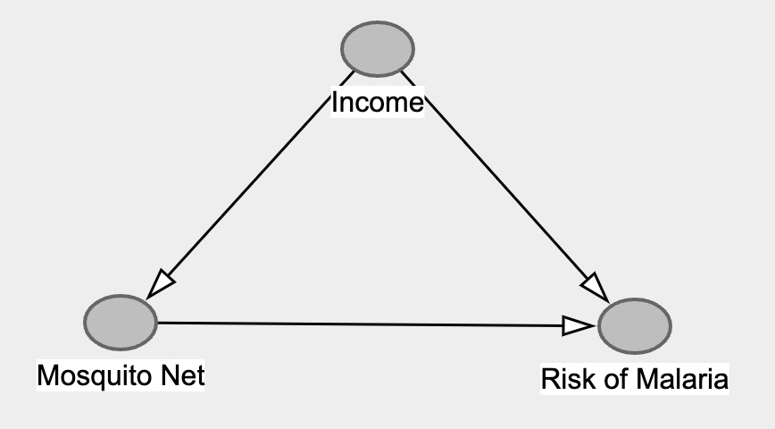
First, use dagitty.net to create this initial dag.
Now, do the two following steps:
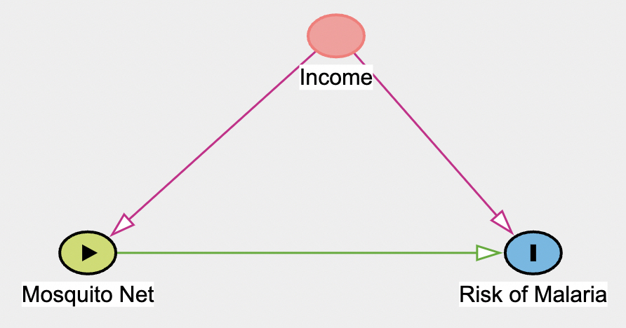
- set Mosquito Net as the “exposure” (aka treatment or independent variable) in Dagitty.
- set Risk of Malaria as the “outcome” (aka response or dependent variable) in Dagitty.
Your DAG should now look like this:
Answer the following four questions:
A. Given the DAG, what type of confound is Income?
B. Given Income’s confound type, if the goal is to find the total effect of Mosquito Nets on the Risk of Malaria, should you include Income as a predictor (aka independent variable) into a regression with Mosquito Nets to explain the Risk of Malaria? Why or why not?
C. Using your Dagitty DAG, find the minimal adjustment set for estimating the total effect of Mosquito Net on Risk of Malaria. How does this compare to part B?
D. Now change the variables in your minimal adjustment set in Part C to “adjusted” on Dagitty. You can do this by selecting the nodes and click the “adjusted” box on the left. After you have completed this, copy and paste your DAG R Code in the chunk below. Be sure to change the chunk parameter from eval=FALSE to eval=TRUE to ensure the code chunk runs.
g <- dagitty::dagitty('
# insert your dagitty copy/paste code here
')
ggdag::ggdag_status(g, text = FALSE, use_labels = "name") +
  guides(color = "none") +  # Turn off legend
  theme_dag()
This is what your DAG above should look like:
Question 2
Let’s now add in more complexity to our DAG.
First, go back and remove “Income” as an “Adjusted” check box.
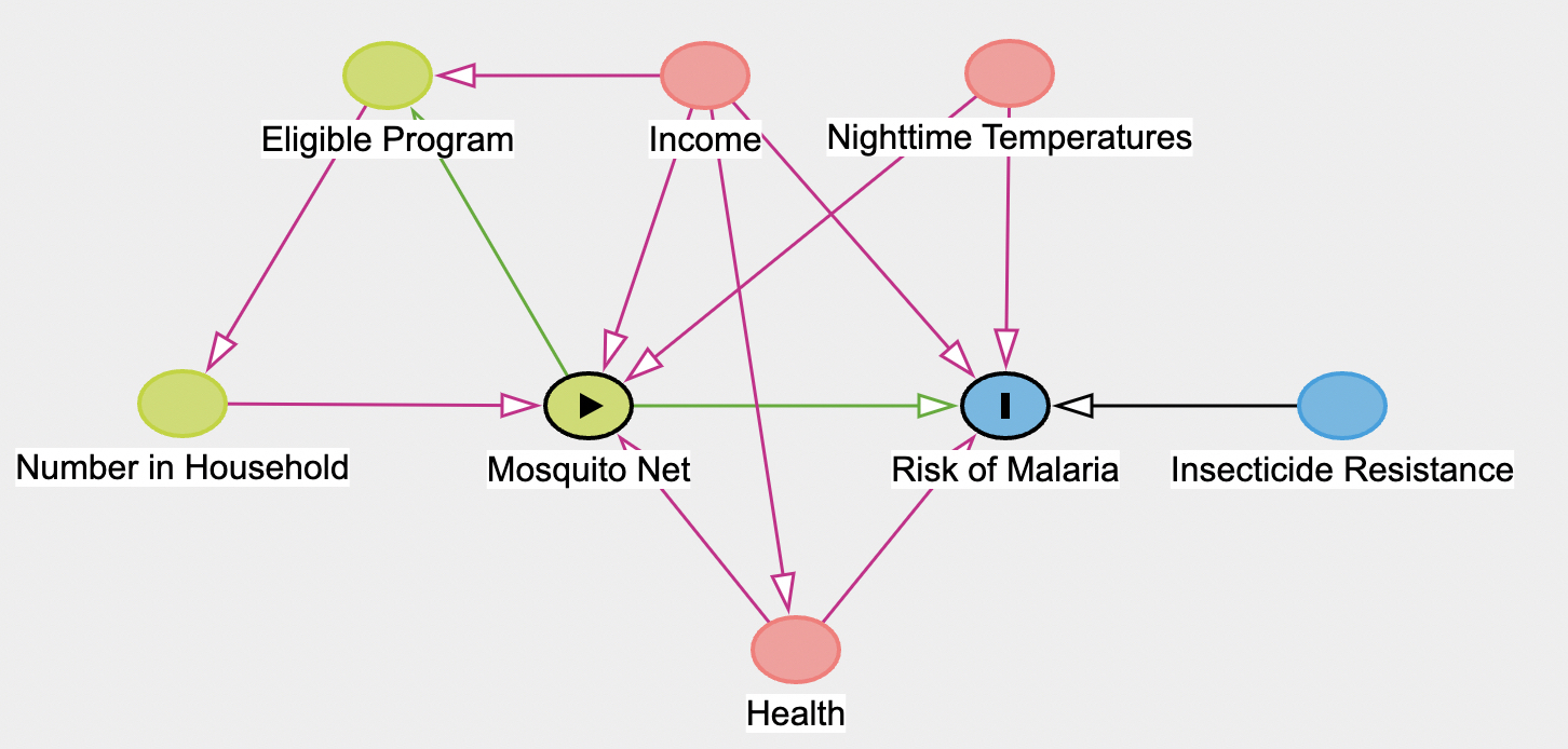
Now, add in additional nodes in your DAG to get the dag above.
Note that in this DAG on “Mosquito Net” (exposure) and “Risk of Malaria” (outcome) have been assigned (i.e., no other nodes are selected as “adjusted”).
Answer the following four questions:
A. Given the DAG, what is the minimal sufficient adjustment sets for estimating the total effect of Mosquito Net on Risk of Malaria?
B. What does this imply for what variables should be included as predictor (independent variables) when trying to identify the total effect of Mosquito Net on Risk of Malaria?
C. Now change the adjustment set nodes to “adjusted” nodes (like in Part D of Q1). After you have completed this, copy and paste your DAG R Code in the chunk below. Be sure to change the chunk parameter from eval=FALSE to eval=TRUE to ensure the code chunk runs.
g <- dagitty::dagitty('
# insert your dagitty copy/paste code here
')
ggdag::ggdag_status(g, text = FALSE, use_labels = "name") +
  guides(color = "none") +  # Turn off legend
  theme_dag()
D. With your new DAG, use dagitty’s adjustment_set() function on your DAG to identify. Confirm that you have the same adjustment set as you found on dagitty.net for Part A.
E. Run dagitty’s ggdag_adjustment_set() function on the g object to get a better graph of the DAG with nodes. Add in these three parameters to your function: shadow = TRUE, use_labels = "label", text = FALSE.
Lecture 6 Examples
In this lab example, we’ll review examples from Lecture 6.
Grandparent and Parent Effect on Child’s Education
Let’s start first with this DAG example used in Lecture 6.
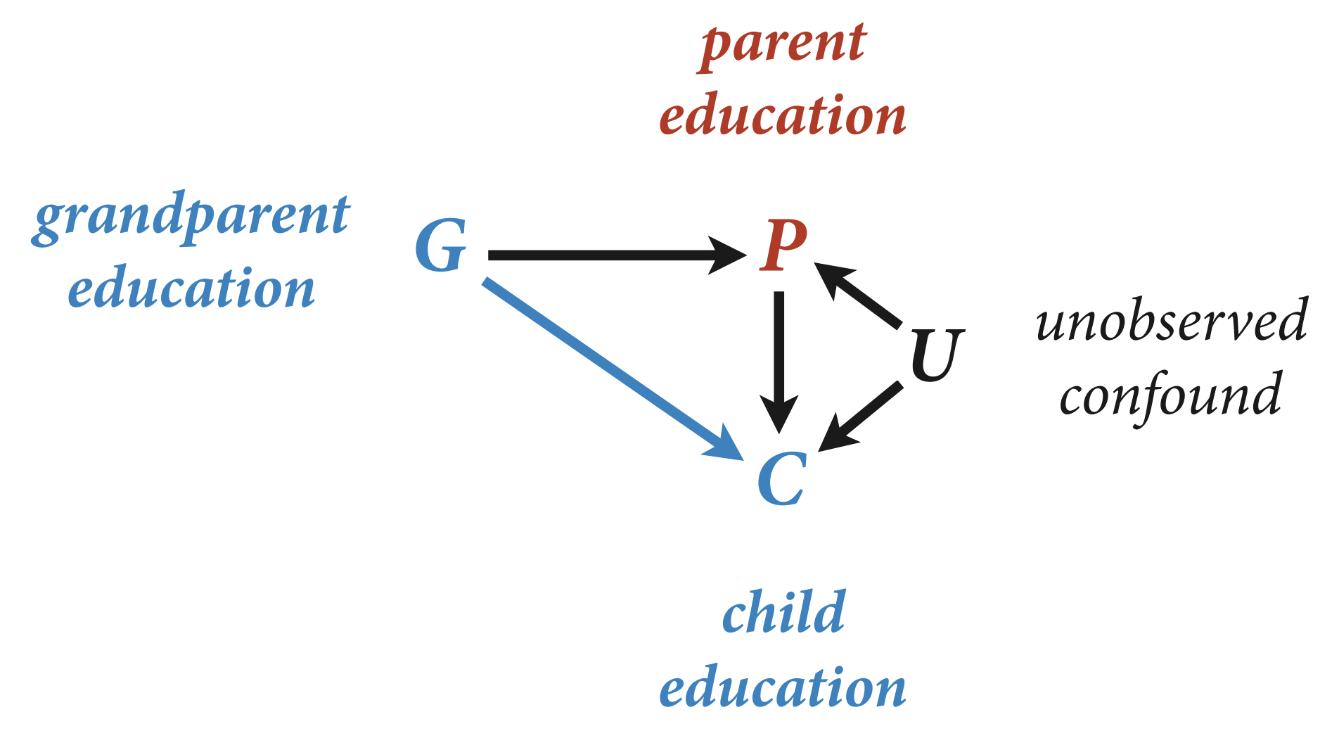
library(rethinking)
N <- 200 # num grandparent-parent-child triads
b_GP <- 1 # direct effect of G on P
b_GC <- 0 # direct effect of G on C
b_PC <- 1 # direct effect of P on C
b_U <- 2 #direct effect of U on P and C
set.seed(1)
# generative model
U <- 2*rbern( N , 0.5 ) - 1
G <- rnorm( N )
P <- rnorm( N , b_GP*G + b_U*U )
C <- rnorm( N , b_PC*P + b_GC*G + b_U*U )
d <- data.frame( C=C , P=P , G=G , U=U )
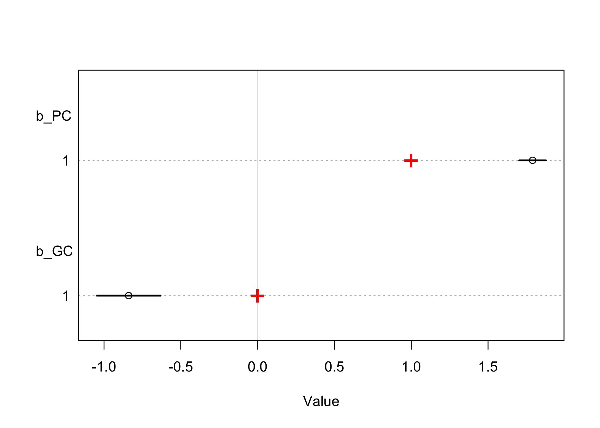
m6.11 <- quap(
alist(
C ~ dnorm( mu , sigma ),
mu <- a + b_PC*P + b_GC*G,
a ~ dnorm( 0 , 1 ),
c(b_PC,b_GC) ~ dnorm( 0 , 1 ),
sigma ~ dexp( 1 )
), data=d )
coeftab_plot(coeftab(m6.11), pars = c("b_PC","b_GC"))
text(x = b_PC, y = 4, "+", col="red", cex = 2) # b_PC
text(x = b_GC, y = 1, "+", col="red", cex = 2) # b_GC
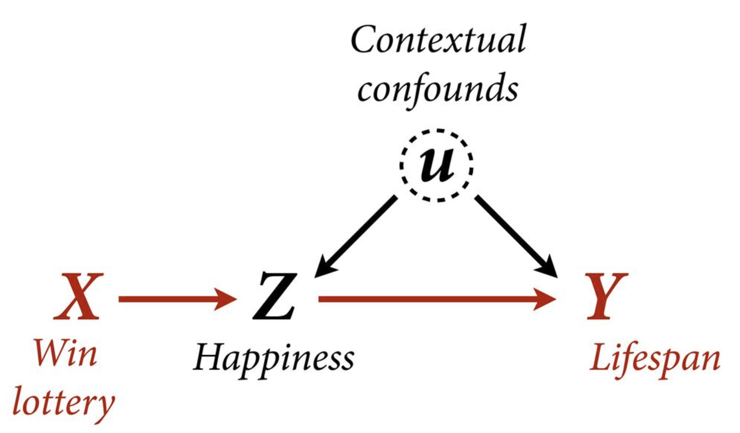
Example
Let’s assume this DAG.
Example 1
Let’s assume this DAG weights:
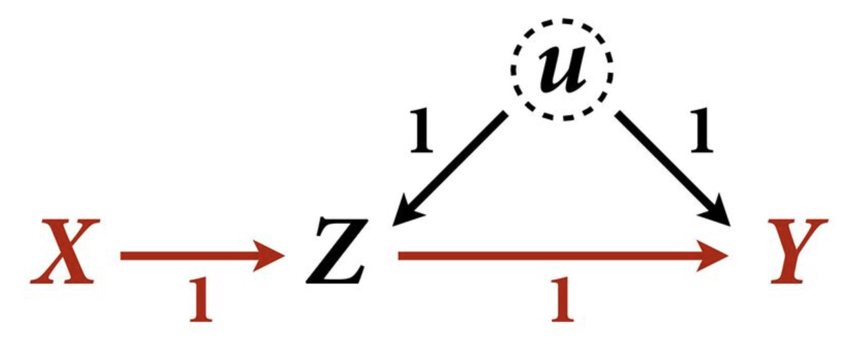
f <- function(n=100,bXZ=1,bZY=1){
  X <- rnorm(n)
  u <- rnorm(n)
  Z <- rnorm(n, bXZ*X + u)
  Y <- rnorm(n, bZY*Z + u)
  bX <- coef( lm(Y ~ X) )['X']
  bXZ <- coef( lm(Y ~ X + Z) )['X']
  return( c(bX,bXZ) )
}

sim <- mcreplicate( 1e4, f(), mc.cores=4)
dens( sim[1,] , lwd=3, xlab="posterior mean", xlim=c(-1,2), ylim=c(0,3) )
dens( sim[2,] , lwd=3, col=2, add=TRUE)
text(x = 0, y = 2.5, "wrong (`Y ~ X + Z`)", col=2, cex = 1)
text(x = 1, y = 1.9, "correct (`Y ~ X`)", col=1, cex = 1)
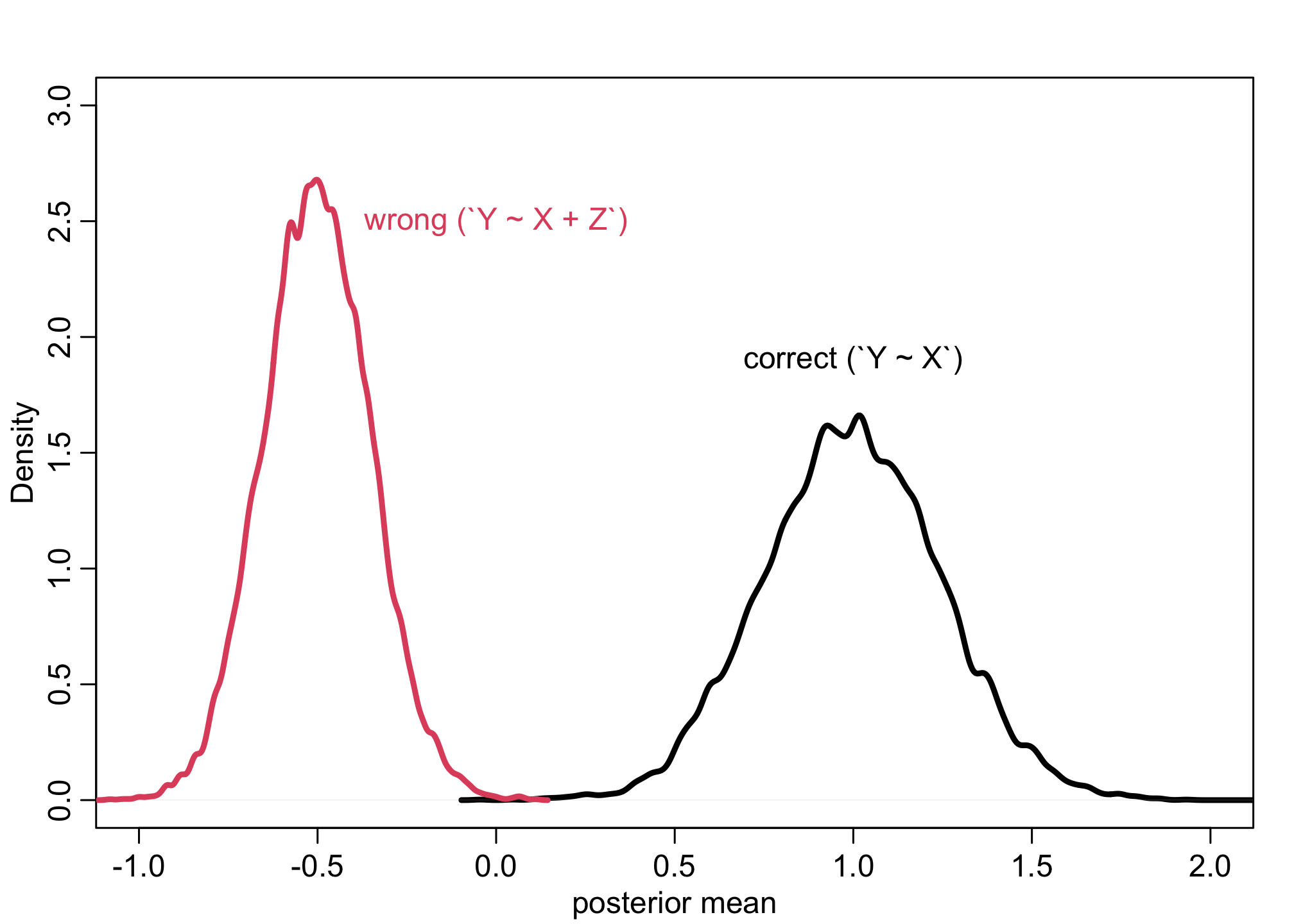
Example 2
f <- function(n=100,bXZ=1,bZY=1){
  X <- rnorm(n)
  u <- rnorm(n)
  Z <- rnorm(n, bXZ*X + u)
  Y <- rnorm(n, bZY*Z + u)
  bX <- coef( lm(Y ~ X) )['X']
  bXZ <- coef( lm(Y ~ X + Z) )['X']
  return( c(bX,bXZ) )
}

sim <- mcreplicate( 1e4, f(bZY=0), mc.cores=4)
dens( sim[1,] , lwd=3, xlab="posterior mean", xlim=c(-1,2), ylim=c(0,3) )
dens( sim[2,] , lwd=3, col=2, add=TRUE)
text(x = -.6, y = 2.8, "wrong (`Y ~ X + Z`)", col=2, cex = 1)
text(x = .5, y = 1.9, "correct (`Y ~ X`)", col=1, cex = 1)
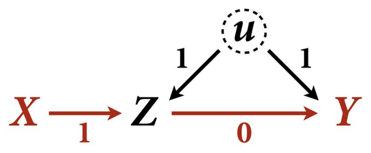
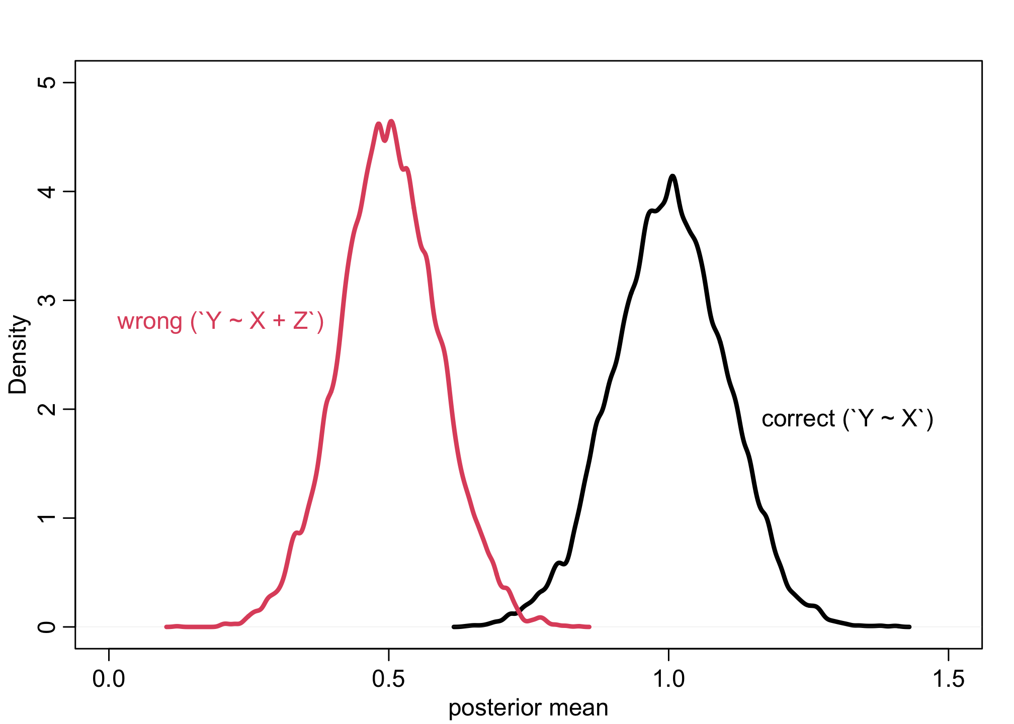
Example 3
f <- function(n=100,bXY=1,bYZ=1) {
 X <- rnorm(n)
 Y <- rnorm(n, bXY*X )
 Z <- rnorm(n, bYZ*Y )
 bX <- coef( lm(Y ~ X) )['X']
 bXZ <- coef( lm(Y ~ X + Z) )['X']
 return( c(bX,bXZ) )
}

sim <- mcreplicate( 1e4 , f() , mc.cores=4 )
dens( sim[1,] , lwd=3 , xlab="posterior mean", xlim=c(0,1.5), ylim=c(0,5)  )
dens( sim[2,] , lwd=3 , col=2 , add=TRUE )
text(x = 0.2, y = 2.8, "wrong (`Y ~ X + Z`)", col=2, cex = 1)
text(x = 1.32, y = 1.9, "correct (`Y ~ X`)", col=1, cex = 1)
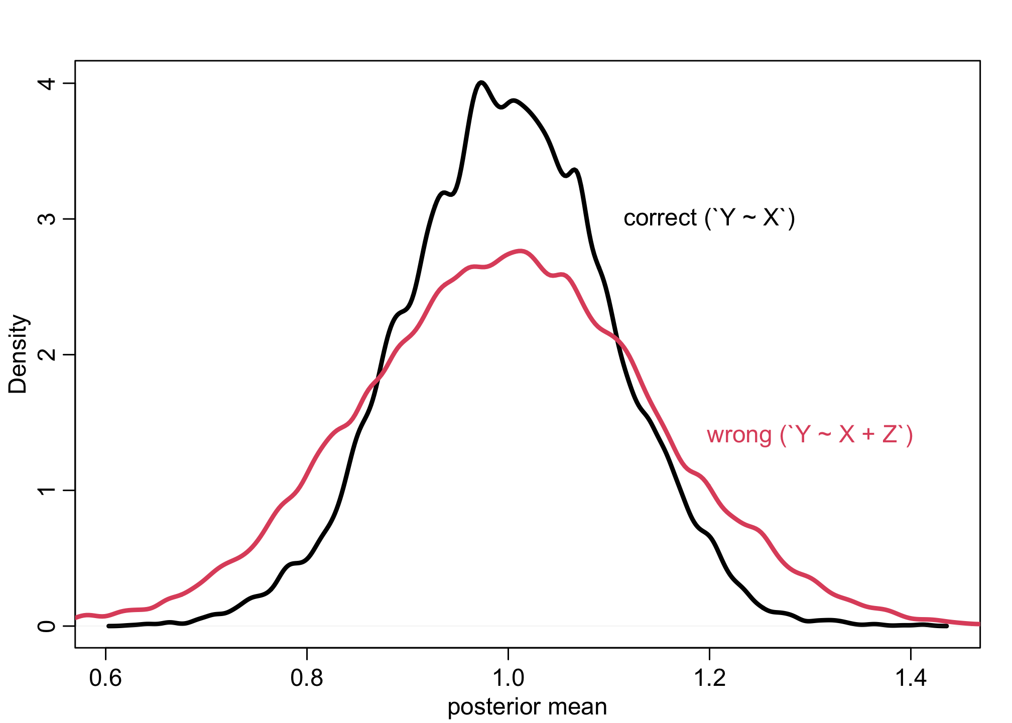
Example 4
 f <- function(n=100,bZX=1,bXY=1) {
 Z <- rnorm(n)
 X <- rnorm(n, bZX*Z )
 Y <- rnorm(n, bXY*X )
 bX <- coef( lm(Y ~ X) )['X']
 bXZ <- coef( lm(Y ~ X + Z) )['X']
 return( c(bX,bXZ) )
}
sim <- mcreplicate( 1e4 , f(n=50) , mc.cores=4 )
dens( sim[1,] , lwd=3 , xlab="posterior mean" )
dens( sim[2,] , lwd=3 , col=2 , add=TRUE )
text(x = 1.3, y = 1.4, "wrong (`Y ~ X + Z`)", col=2, cex = 1)
text(x = 1.2, y = 3, "correct (`Y ~ X`)", col=1, cex = 1)
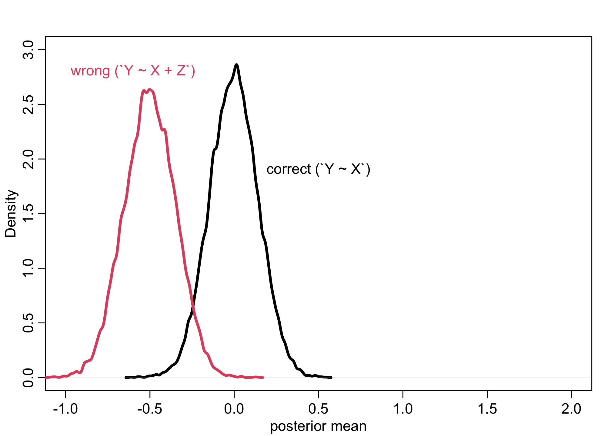
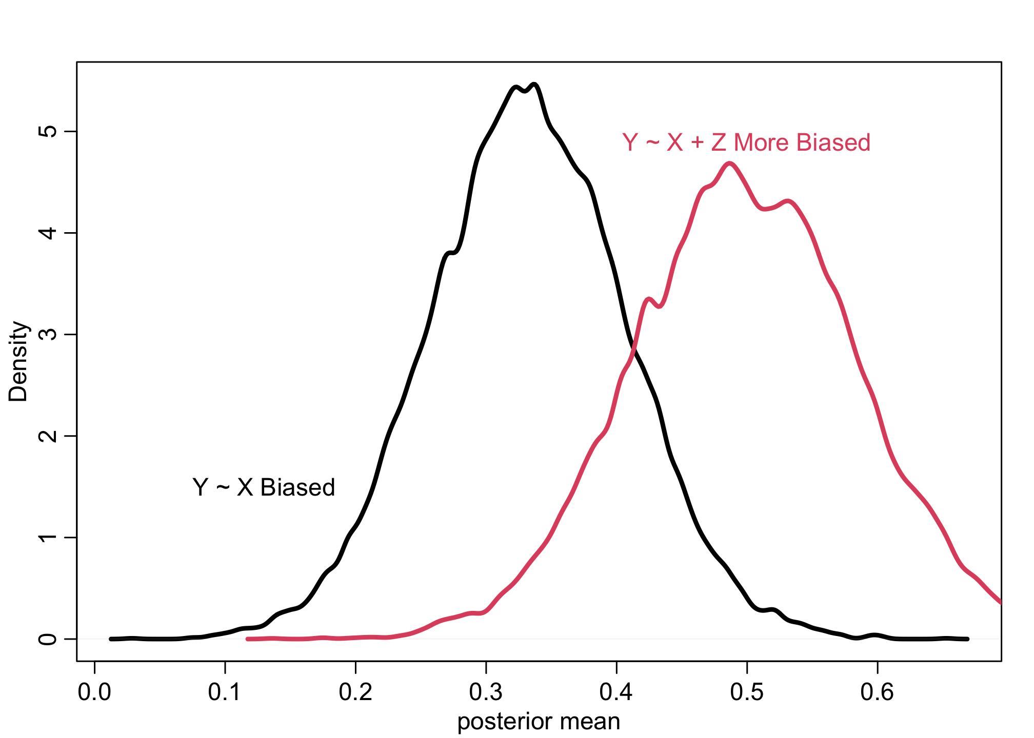
Example 5
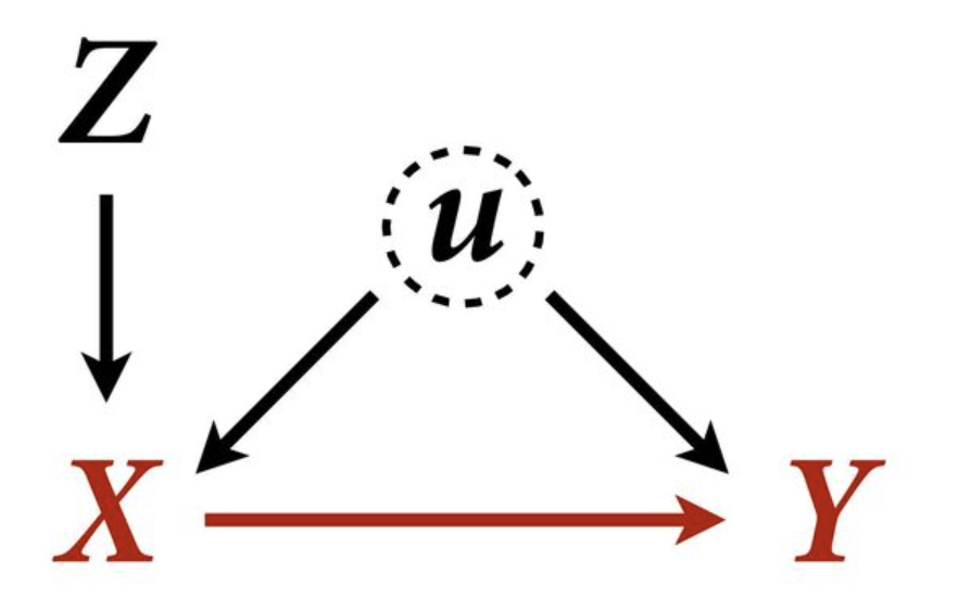
f <- function(n=100,bZX=1,bXY=1) {
 Z <- rnorm(n)
 u <- rnorm(n)
 X <- rnorm(n, bZX*Z + u )
 Y <- rnorm(n, bXY*X + u )
 bX <- coef( lm(Y ~ X) )['X']
 bXZ <- coef( lm(Y ~ X + Z) )['X']
 return( c(bX,bXZ) )
}
sim <- mcreplicate( 1e4 , f(bXY=0) , mc.cores=8 )
dens( sim[1,] , lwd=3 , xlab="posterior mean" )
dens( sim[2,] , lwd=3 , col=2 , add=TRUE )
text(x = 0.5, y = 4.9, "Y ~ X + Z More Biased", col=2, cex = 1)
text(x = 0.13, y = 1.5, "Y ~ X Biased", col=1, cex = 1)
Package versions
sessionInfo()
## R version 4.1.1 (2021-08-10)
## Platform: aarch64-apple-darwin20 (64-bit)
## Running under: macOS Monterey 12.1
##
## Matrix products: default
## BLAS:   /Library/Frameworks/R.framework/Versions/4.1-arm64/Resources/lib/libRblas.0.dylib
## LAPACK: /Library/Frameworks/R.framework/Versions/4.1-arm64/Resources/lib/libRlapack.dylib
##
## locale:
## [1] en_US.UTF-8/en_US.UTF-8/en_US.UTF-8/C/en_US.UTF-8/en_US.UTF-8
##
## attached base packages:
## [1] parallel  stats     graphics  grDevices datasets  utils     methods
## [8] base
##
## other attached packages:
## [1] rethinking_2.21      cmdstanr_0.4.0.9001  rstan_2.21.3
## [4] ggplot2_3.3.5        StanHeaders_2.21.0-7
##
## loaded via a namespace (and not attached):
##  [1] sass_0.4.0           jsonlite_1.7.2       bslib_0.3.1
##  [4] RcppParallel_5.1.4   assertthat_0.2.1     posterior_1.1.0
##  [7] distributional_0.2.2 highr_0.9            stats4_4.1.1
## [10] tensorA_0.36.2       renv_0.14.0          yaml_2.2.1
## [13] pillar_1.6.4         backports_1.4.1      lattice_0.20-44
## [16] glue_1.6.0           uuid_1.0-3           digest_0.6.29
## [19] checkmate_2.0.0      colorspace_2.0-2     htmltools_0.5.2
## [22] pkgconfig_2.0.3      bookdown_0.24        purrr_0.3.4
## [25] mvtnorm_1.1-3        scales_1.1.1         processx_3.5.2
## [28] tibble_3.1.6         generics_0.1.1       farver_2.1.0
## [31] ellipsis_0.3.2       withr_2.4.3          cli_3.1.0
## [34] mime_0.12            magrittr_2.0.1       crayon_1.4.2
## [37] evaluate_0.14        ps_1.6.0             fs_1.5.0
## [40] fansi_0.5.0          MASS_7.3-54          pkgbuild_1.3.1
## [43] blogdown_1.5         tools_4.1.1          loo_2.4.1
## [46] prettyunits_1.1.1    lifecycle_1.0.1      matrixStats_0.61.0
## [49] stringr_1.4.0        munsell_0.5.0        callr_3.7.0
## [52] compiler_4.1.1       jquerylib_0.1.4      rlang_0.4.12
## [55] grid_4.1.1           rstudioapi_0.13      base64enc_0.1-3
## [58] rmarkdown_2.11       xaringanExtra_0.5.5  gtable_0.3.0
## [61] codetools_0.2-18     inline_0.3.19        abind_1.4-5
## [64] DBI_1.1.1            R6_2.5.1             gridExtra_2.3
## [67] lubridate_1.8.0      knitr_1.36           dplyr_1.0.7
## [70] fastmap_1.1.0        utf8_1.2.2           downloadthis_0.2.1
## [73] bsplus_0.1.3         shape_1.4.6          stringi_1.7.6
## [76] Rcpp_1.0.7           vctrs_0.3.8          tidyselect_1.1.1
## [79] xfun_0.28            coda_0.19-4