Class 4

Introduction

For this class, we’ll review code examples found in Chapter 4 and some of Chapter 5.

Chapter 4: The causes aren’t in the data

This chapter expanded regression to multiple regression. This is when we consider more than 1 predictor (independent) variable. We’ll consider a new categorical variable of sex.

Total causal effect of S on W

set.seed(100) # fyi, in code seed wasn't set so may be slightly different
library(rethinking)
data("Howell1")
d <- Howell1[Howell1$age>=18,]

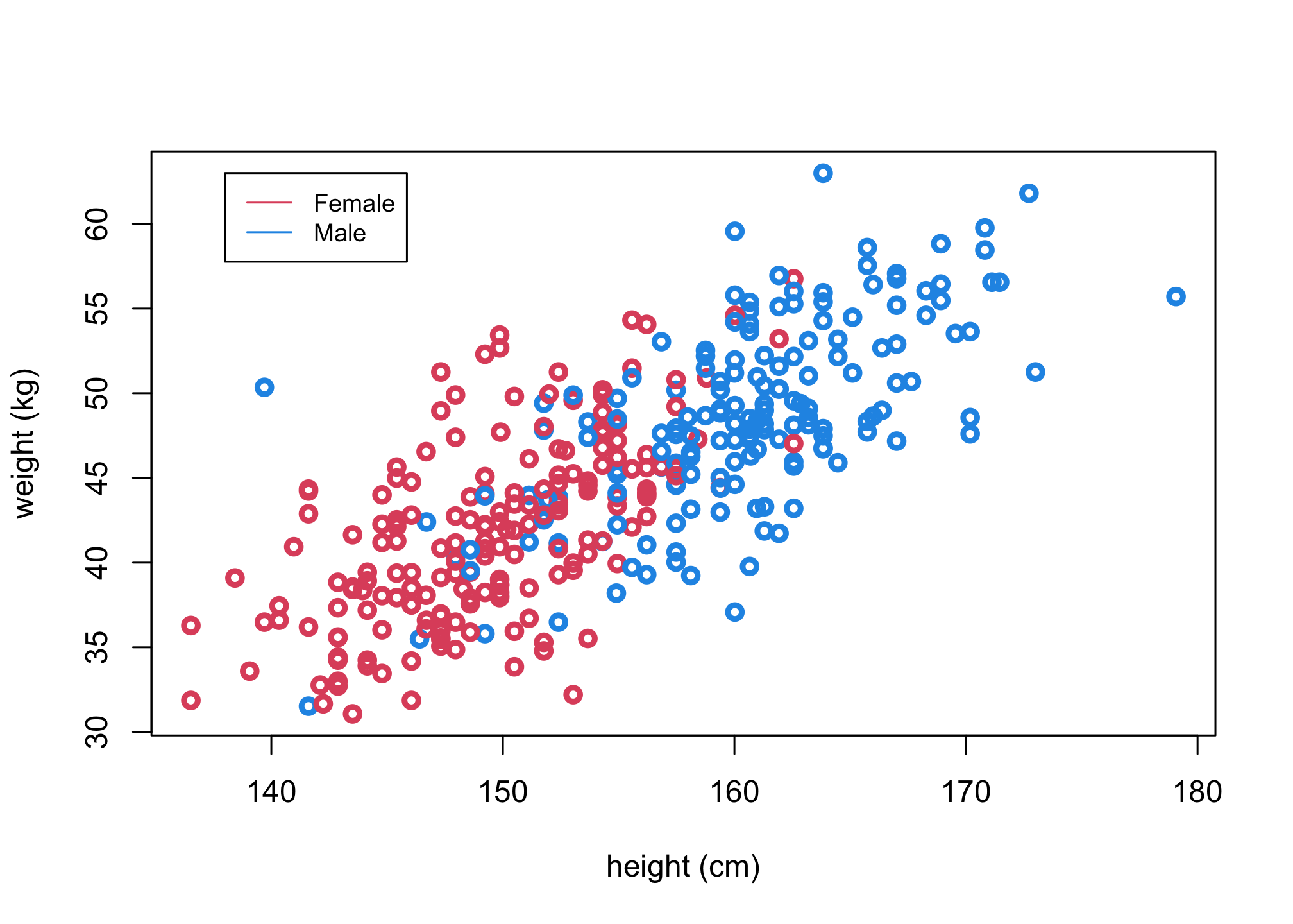
Let’s again consider the 18+ year old from the Howell dataset, but now look at the role of a third variable: sex.

plot(d$height, d$weight, col = ifelse(d$male,4,2),  xlab = "height (cm)", ylab = "weight (kg)",  lwd=3)
legend(138, 63, legend=c("Female", "Male"),
       col=c(2,4), lty=1:1, cex=0.8)

head(d)

##    height   weight age male
## 1 151.765 47.82561  63    1
## 2 139.700 36.48581  63    0
## 3 136.525 31.86484  65    0
## 4 156.845 53.04191  41    1
## 5 145.415 41.27687  51    0
## 6 163.830 62.99259  35    1

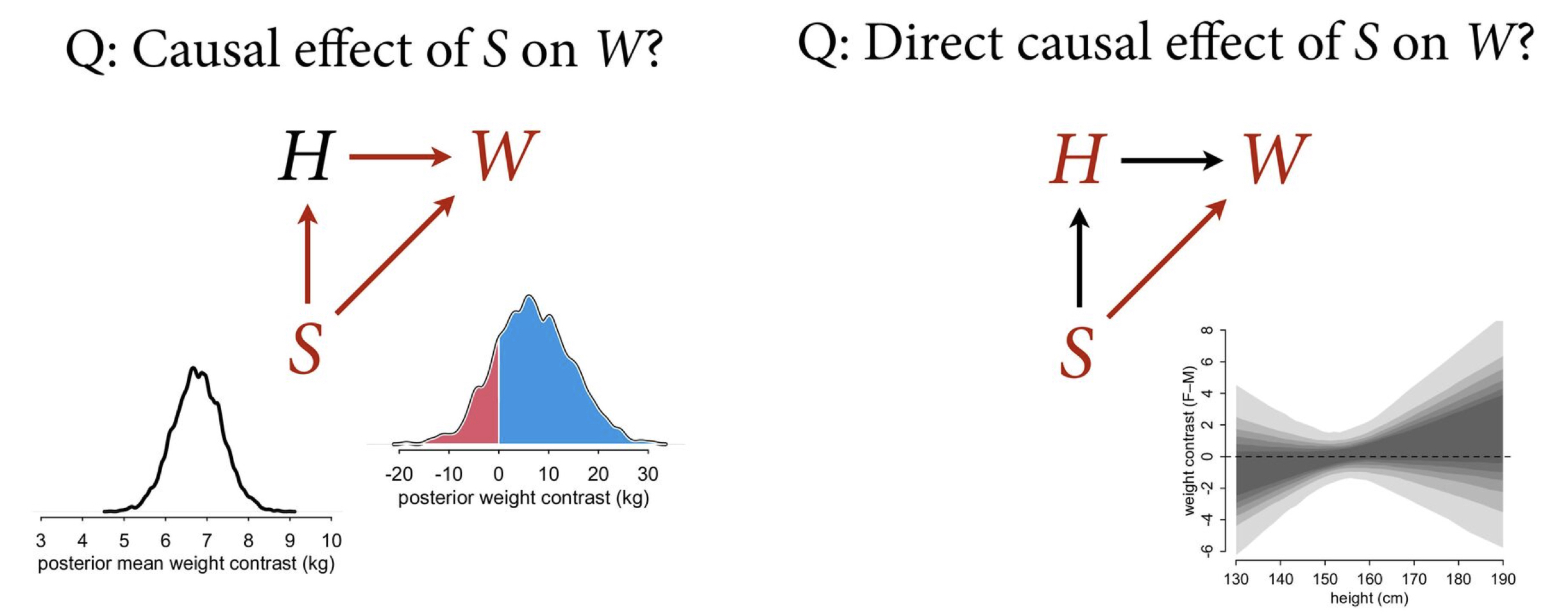
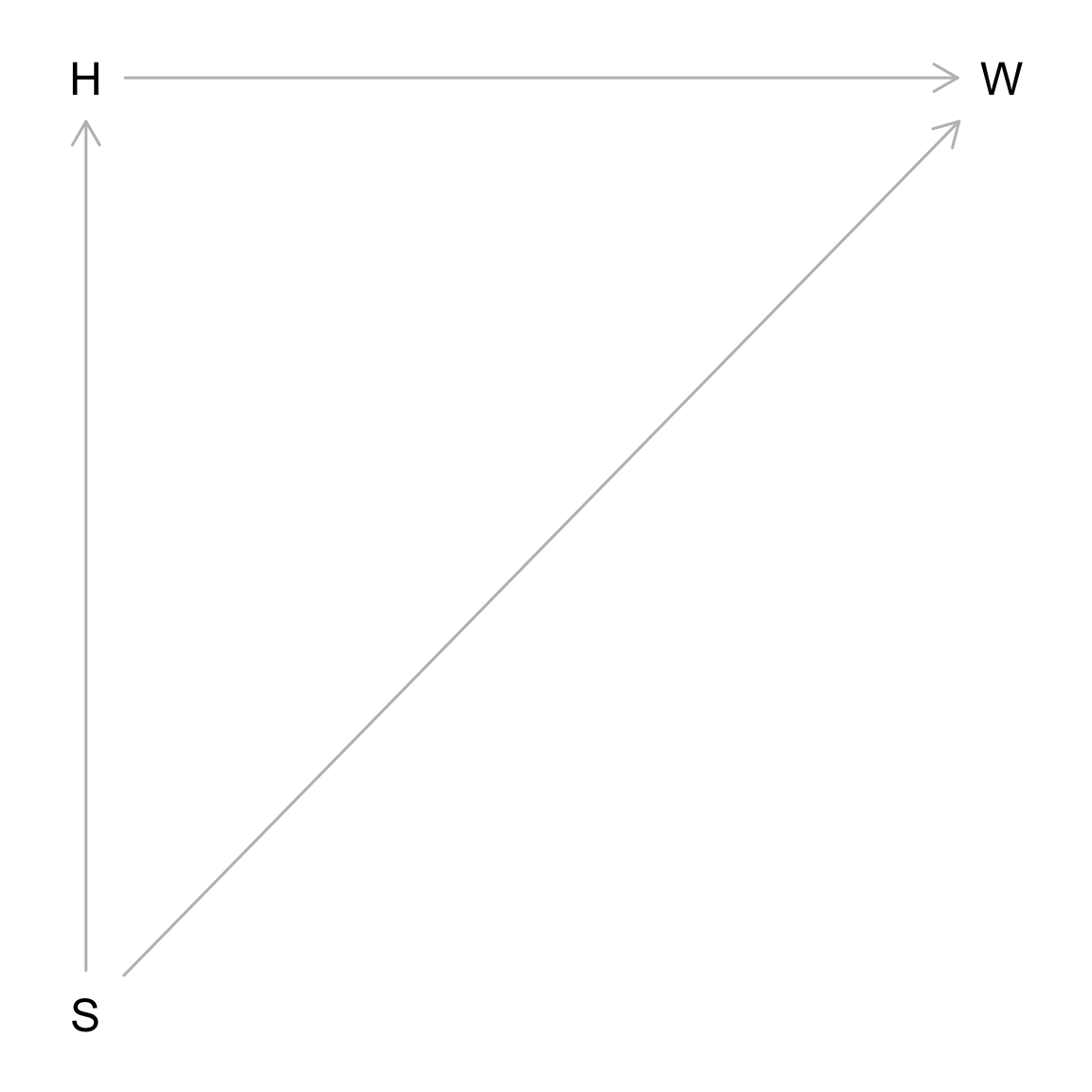
We are interested in the total causal effect of S on W (i.e., through both paths direct and via H).

library(dagitty)

g <- dagitty('dag {
bb="0,0,1,1"
S [pos="0.251,0.481"]
H [pos="0.251,0.352"]
W [pos="0.481,0.352"]
S -> H
S -> W
H -> W
}
')
plot(g)

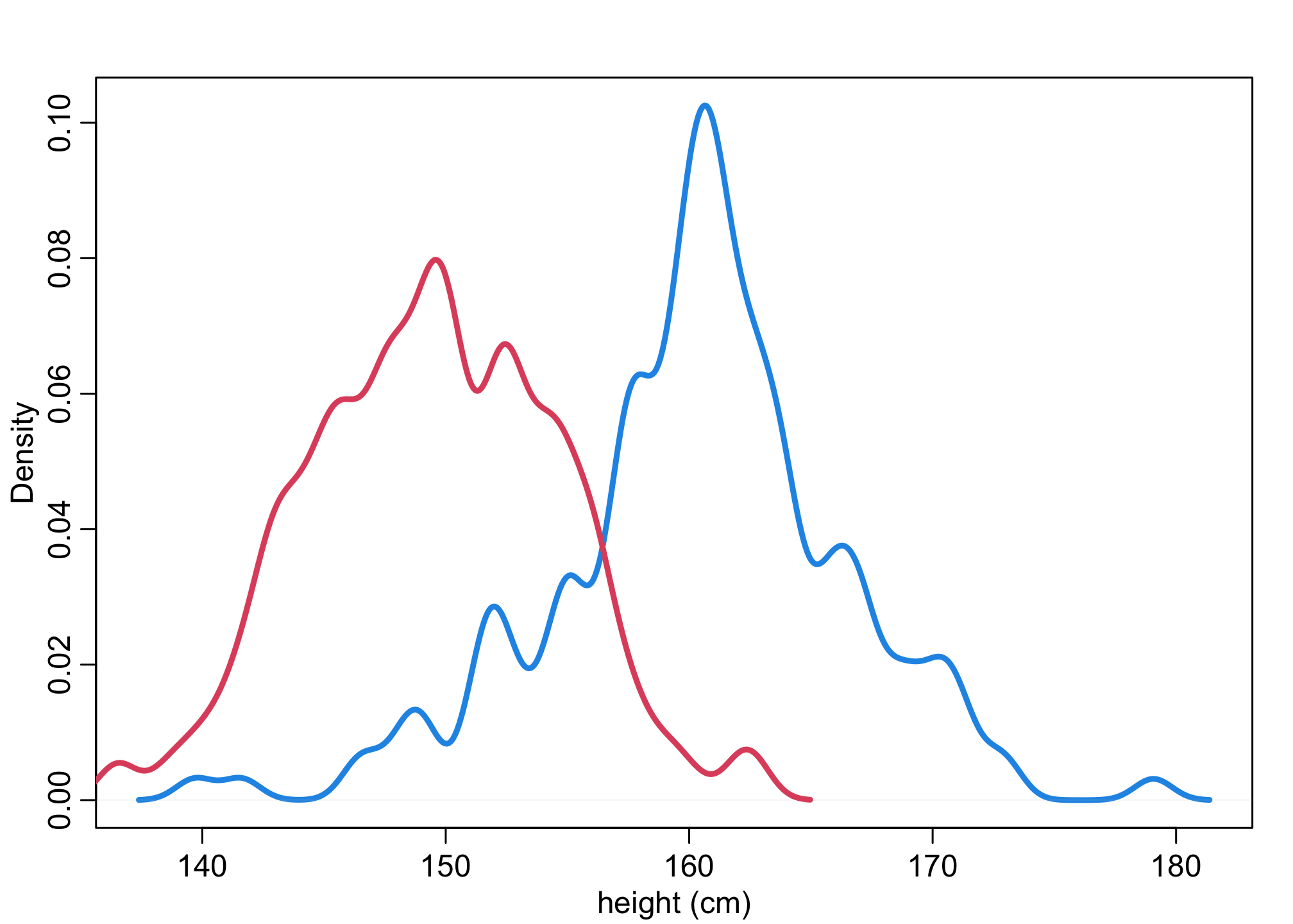
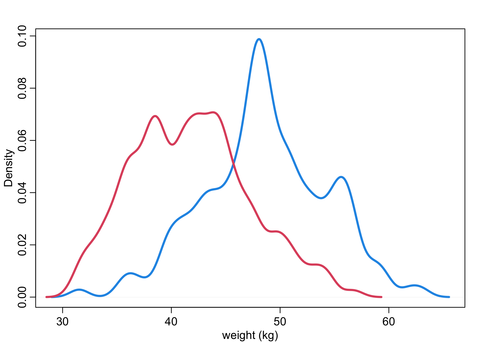
Let’s first look at the distributions of heights and weights by sex.

# new height, weight, sex categorical variable example
dens(d$height[d$male==1],lwd=3,col=4,xlab="height (cm)")
dens(d$height[d$male==0],lwd=3,col=2,add=TRUE)

dens(d$weight[d$male==1],lwd=3,col=4,xlab="weight (kg)")
dens(d$weight[d$male==0],lwd=3,col=2,add=TRUE)

Causal effect of S on W?

See model in Lecture 4.

# W ~ S
dat <- list(
    W = d$weight,
    S = d$male + 1 ) # S=1 female, S=2 male

m_SW <- quap(
    alist(
        W ~ dnorm(mu,sigma),
        mu <- a[S],
        a[S] ~ dnorm(60,10), # assume both sexes have same priors
        sigma ~ dunif(0,10)
    ), data=dat )

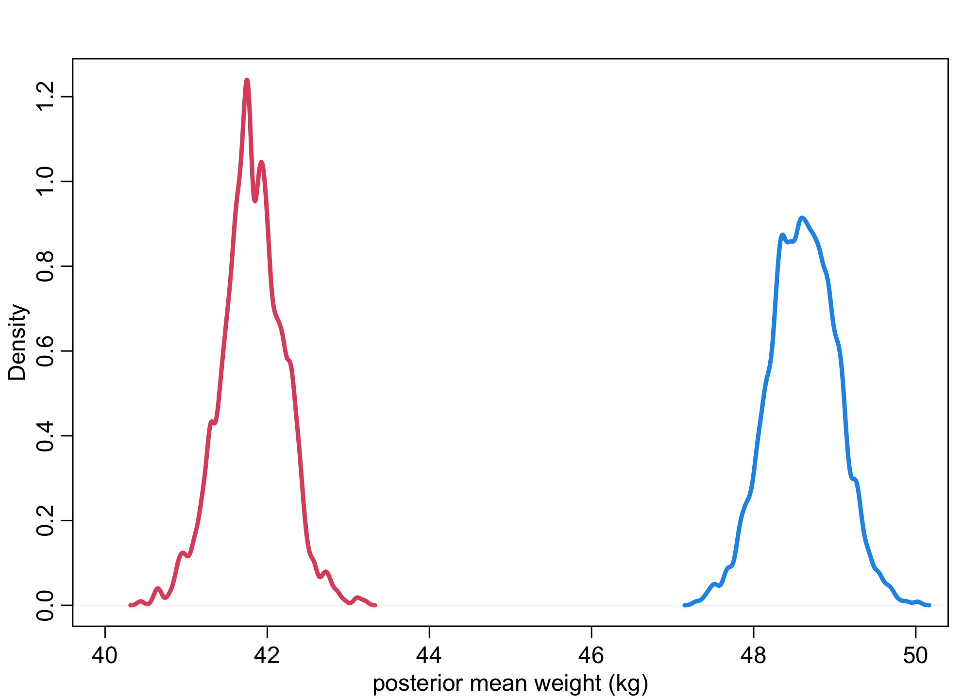
First thing we’ll do is calculate the posterior mean weights (Lecture 4).

N_sim = 1000 # number of samples

# posterior means
post <- extract.samples(m_SW, n = N_sim)
dens( post$a[,1] , xlim=c(39,50) , lwd=3 , col=2 , xlab="posterior mean weight (kg)" )
dens( post$a[,2] , lwd=3 , col=4 , add=TRUE )

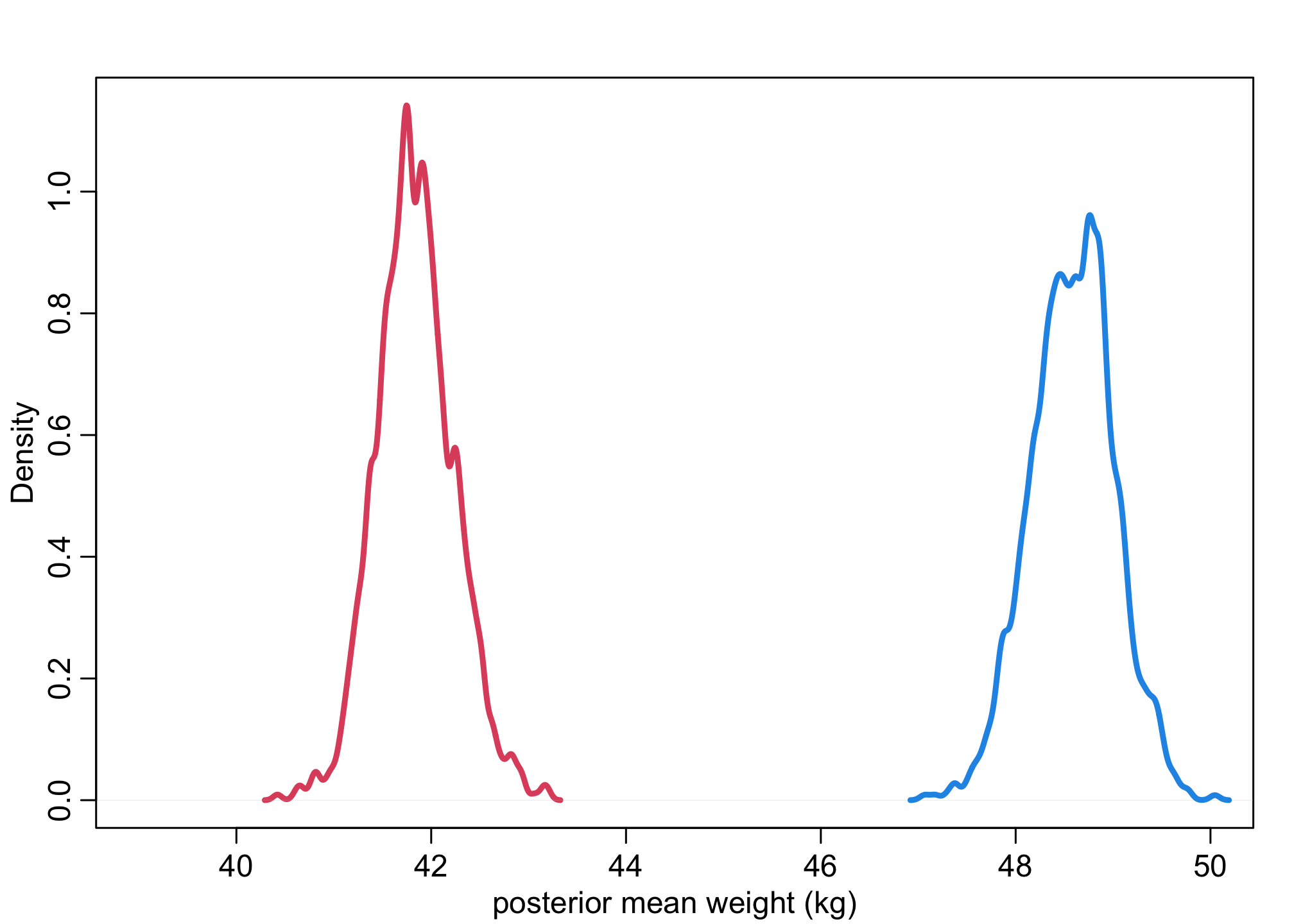
We can then calculate the posterior mean weight contrast.

# causal contrast (in means)
mu_contrast <- post$a[,2] - post$a[,1]
dens( mu_contrast , xlim=c(3,10) , lwd=3 , col=1 , xlab="posterior mean weight contrast (kg)" )

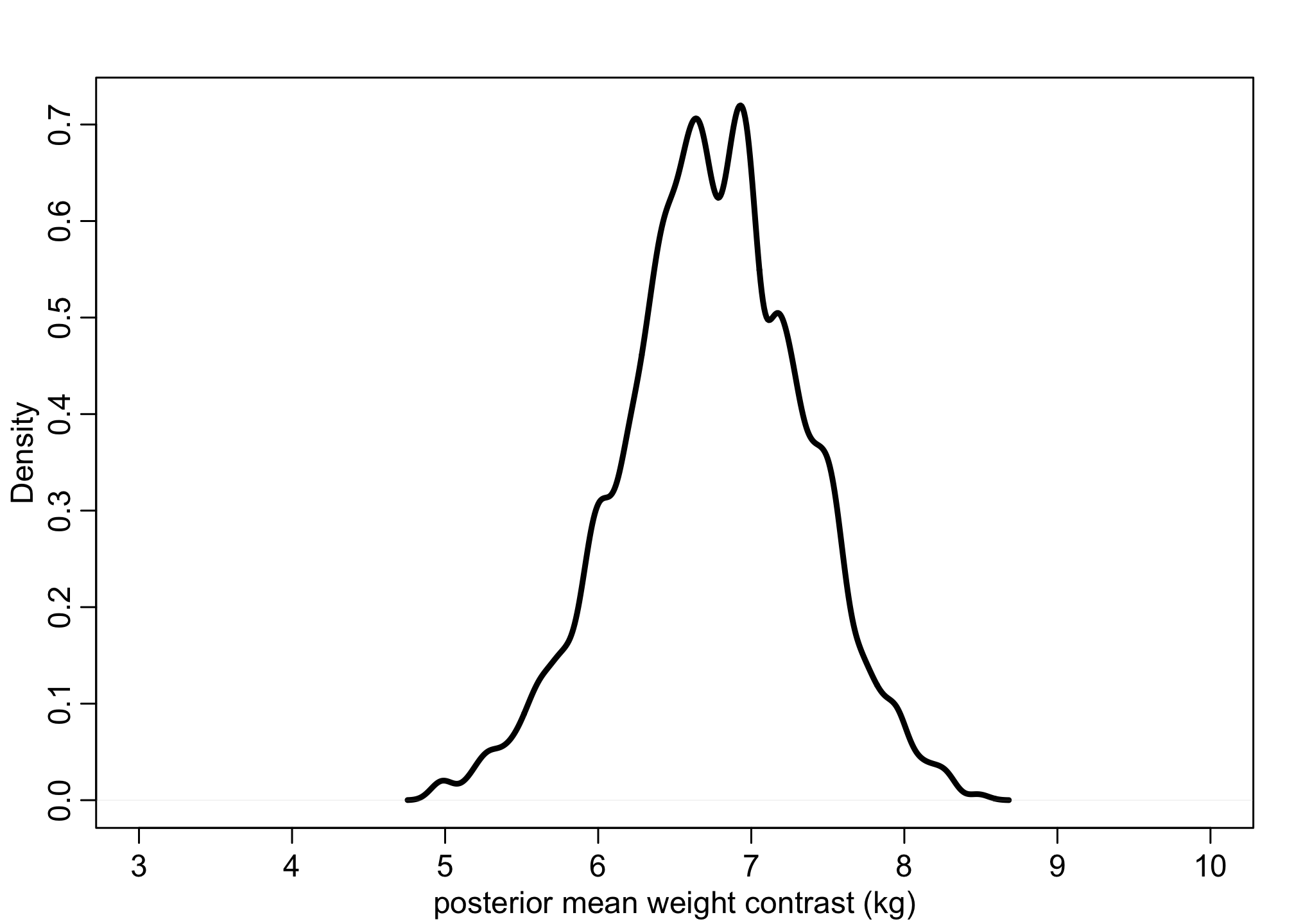
On average, men are heavily on average but not necessarily reliably heavier.

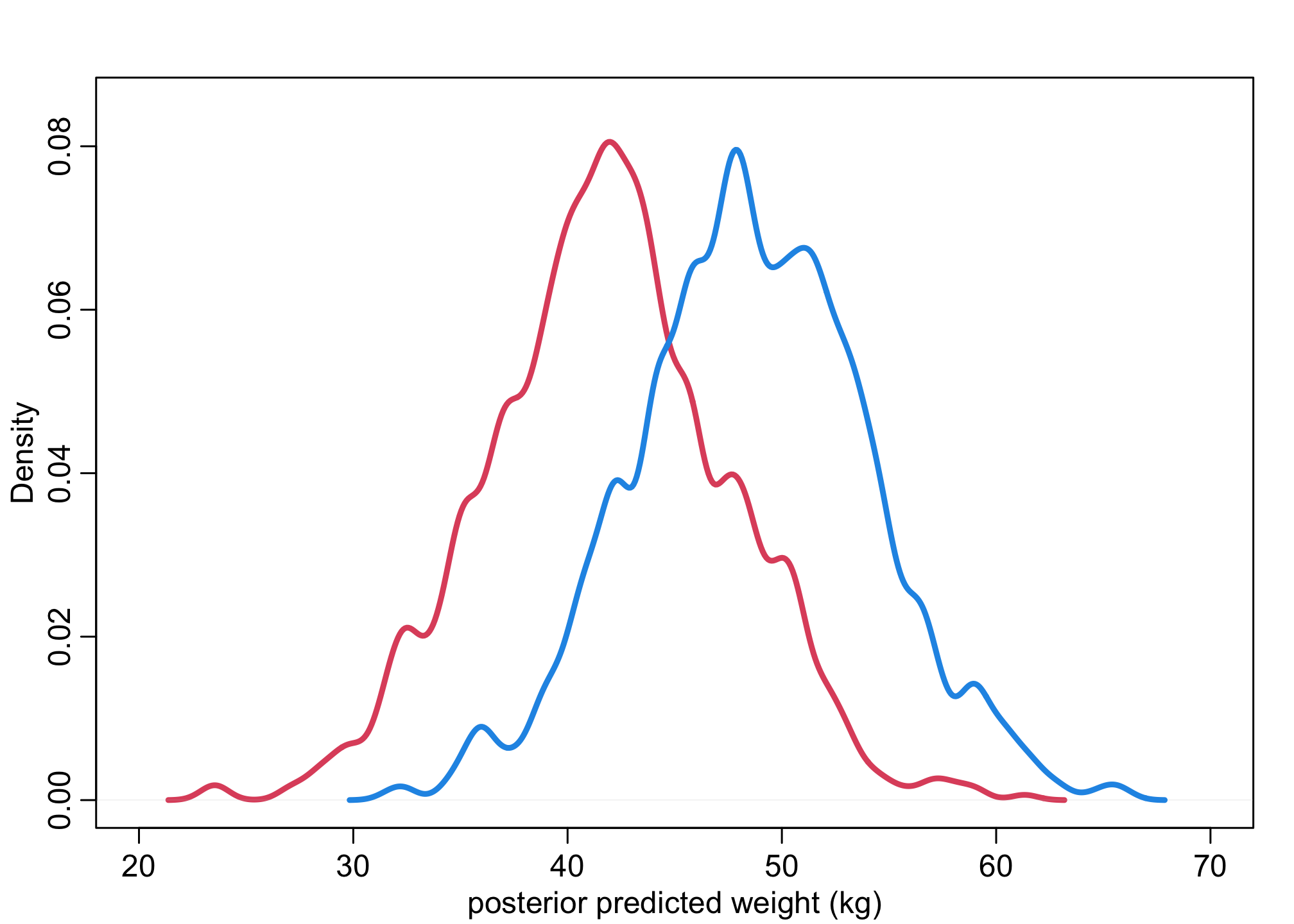
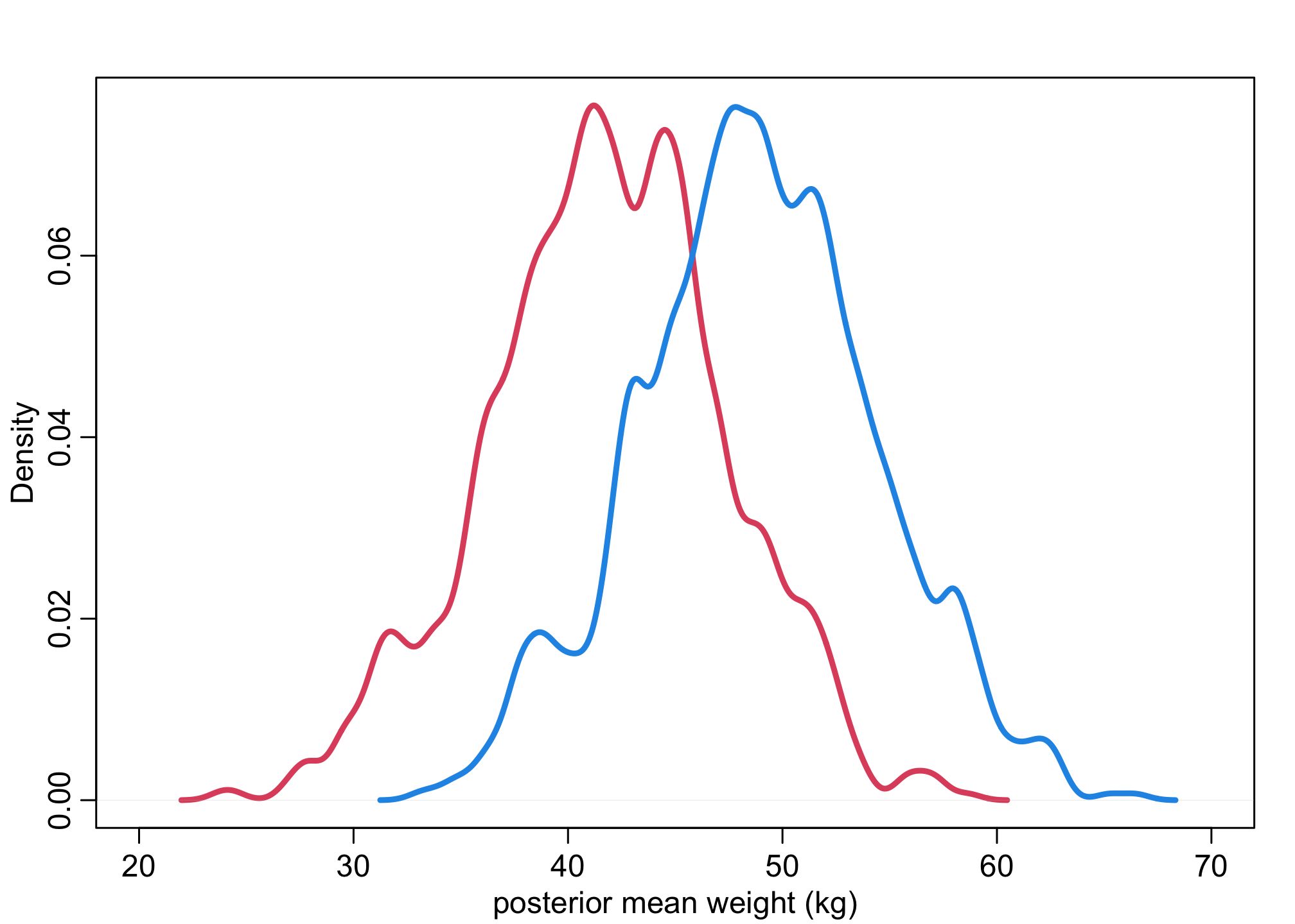
Next, we’ll generate predictive weights. This allows us to calculate the contrast on the individual level.

N_sim = 1000 # let's do 1,000 samples

# posterior W distributions
W1 <- rnorm( N_sim , post$a[,1] , post$sigma )
W2 <- rnorm( N_sim , post$a[,2] , post$sigma )
dens( W1 , xlim=c(20,70) , ylim=c(0,0.085) , lwd=3 , col=2 , xlab="posterior predicted weight (kg)" )
dens( W2 , lwd=3 , col=4 , add=TRUE )

# W contrast
W_contrast <- W2 - W1
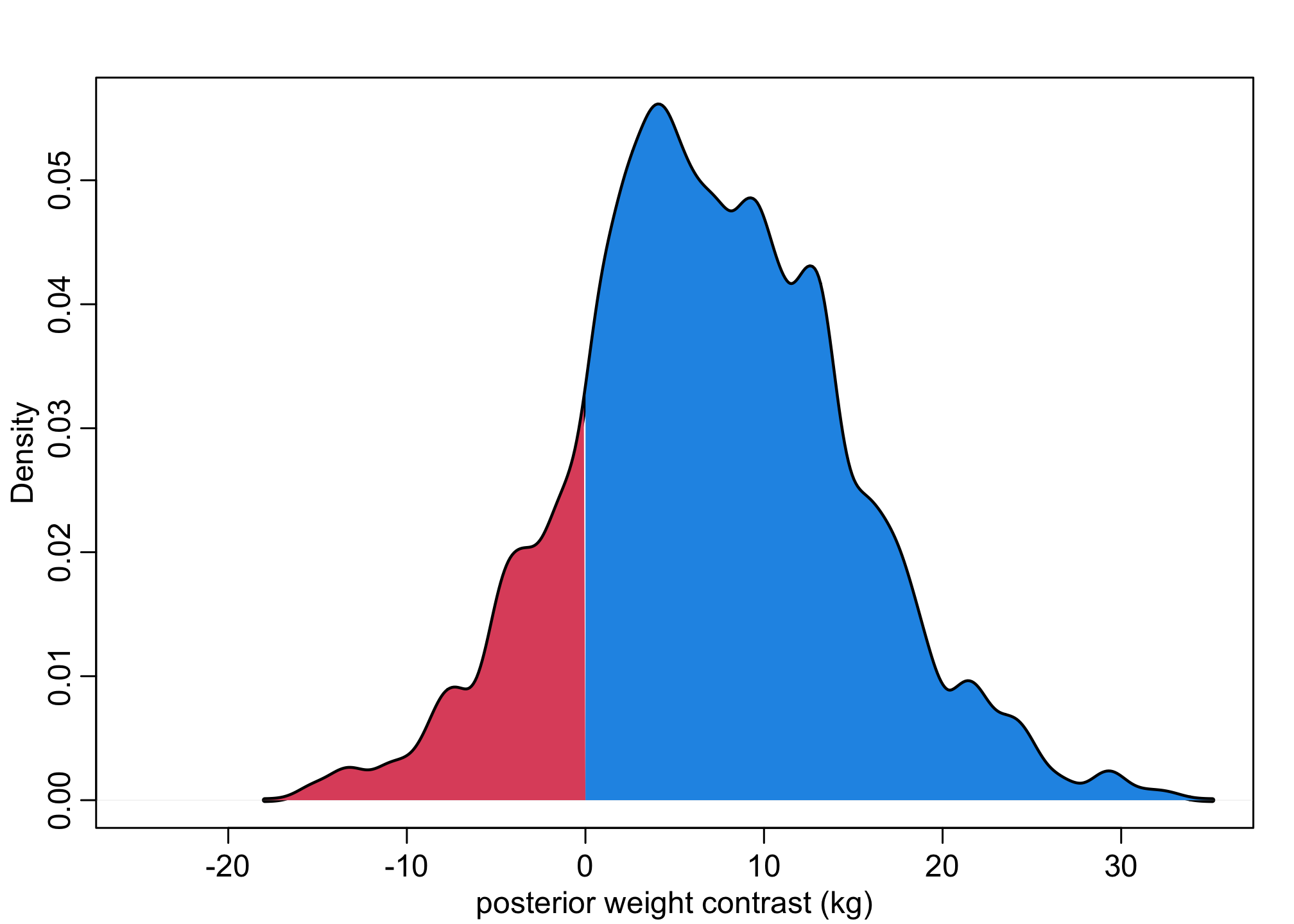
dens( W_contrast , xlim=c(-25,35) , lwd=3 , col=1 , xlab="posterior weight contrast (kg)" )

Wdens <- density(W_contrast,adj=0.5)
polygon(c(Wdens$x[Wdens$x>0], max(Wdens$x), 0), c(Wdens$y[Wdens$x>0], 0, 0), col = 4, border = NA )
polygon(c(Wdens$x[Wdens$x<0], 0, min(Wdens$x)), c(Wdens$y[Wdens$x<0], 0, 0), col = 2, border = NA )

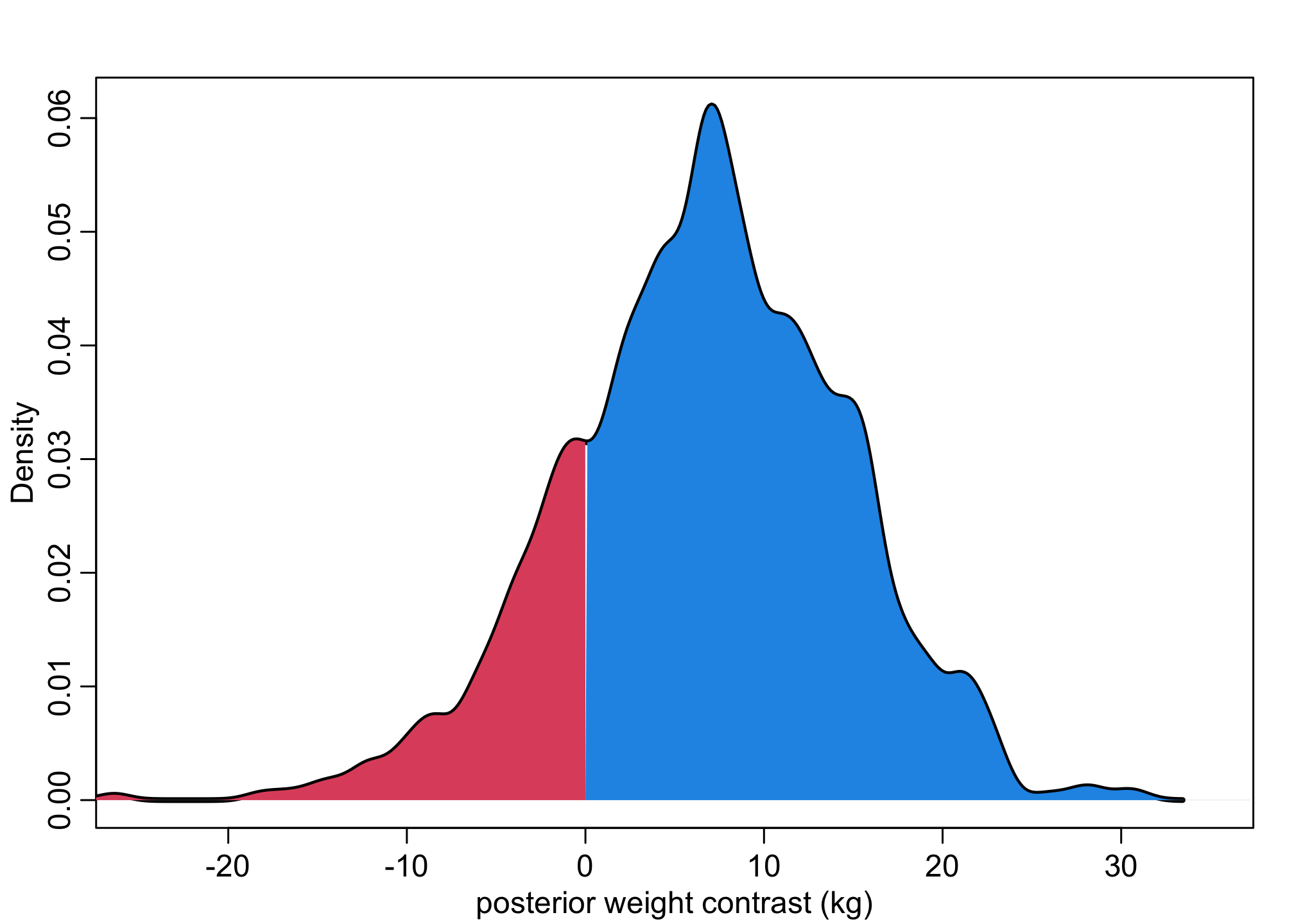
This allows us to calculate how many cases where men are heavier (above zero) and are lighter (below zero).

# proportion above zero
sum( W_contrast > 0 ) / N_sim

## [1] 0.808

# proportion below zero
sum( W_contrast < 0 ) / N_sim

## [1] 0.192

About 82% the males are heavier than the women – but about 20% of cases women are lighter

Why is the posterior contrasts not exactly equal to the lecture?

What would happen if you increase number of samples to 100,000? what about 1,000,000 (only run if you have sufficient RAM)?

Alternative Approach

An alternative approach for calculating the contrast using the link() and sim() functions.

we can use extract.samples similarly as link()
can also use extracted samples to calculate similar function to sim()

First, since we’re considering the mean (mu) value, we can use the link() function.

# approach 2: use link function
N_sim = 1000

muF <- link(m_SW,data=list(S=1), N_sim)
muM <- link(m_SW,data=list(S=2), N_sim)

dens( muF , xlim=c(40,50) , lwd=3 , col=2 , xlab="posterior mean weight (kg)" )
dens( muM , lwd=3 , col=4 , add=TRUE )

# causal contrast (in means)
link_contrast <- muM - muF
dens( mu_contrast , xlim=c(3,10) , lwd=3 , col=1 , xlab="posterior mean weight contrast (kg)") # red using extract.samples
lines( density(link_contrast) , lwd=3 , col=2 ) # black is link()

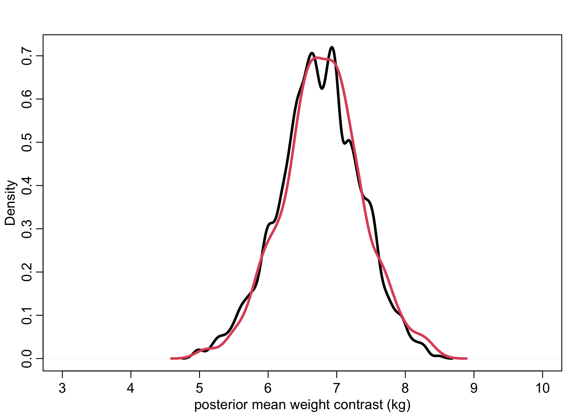
Notice this is nearly identical to the earlier charts with using extract.samples. We can follow a similar logic but look at the posterior predictives.

muF <- sim(m_SW,data=list(S=1), N_sim)
muM <- sim(m_SW,data=list(S=2), N_sim)

dens( muF , xlim=c(20,70) , lwd=3 , col=2 , xlab="posterior mean weight (kg)" )
dens( muM , lwd=3 , col=4 , add=TRUE )

contrast <- muM - muF

dens( contrast , xlim=c(-25,35) , lwd=3 , col=1 , xlab="posterior weight contrast (kg)" )

Wdens <- density(contrast,adj=0.5)
polygon(c(Wdens$x[Wdens$x>0], max(Wdens$x), 0), c(Wdens$y[Wdens$x>0], 0, 0), col = 4, border = NA )
polygon(c(Wdens$x[Wdens$x<0], 0, min(Wdens$x)), c(Wdens$y[Wdens$x<0], 0, 0), col = 2, border = NA )

# proportion above zero
sum( contrast > 0 ) / N_sim

## [1] 0.839

# proportion below zero
sum( contrast < 0 ) / N_sim

## [1] 0.161

What would happen if you increase number of samples for link() and sim()?

How does the computational speed compare for using extract.samples() vs. link() / sim()?

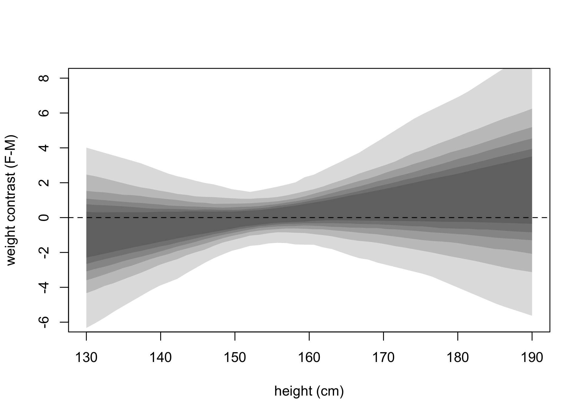
Direct causal effect of S on W?

We can also try to measure the sole effect of S on W. From about minute 37 in Lecture 4.

In this we stratify by sex where we will get an intercept and a slope unique for each of the sexes.

# W ~ S + H
dat <- list(
    W = d$weight,
    H = d$height,
    Hbar = mean(d$height),
    S = d$male + 1 ) # S=1 female, S=2 male

m_SHW <- quap(
    alist(
        W ~ dnorm(mu,sigma),
        mu <- a[S] + b[S]*(H-Hbar),
        a[S] ~ dnorm(60,10),
        b[S] ~ dlnorm(0,1),
        sigma ~ dunif(0,10)
    ), data=dat )

Let’s now get the posterior predictives for the contrasts.

xseq <- seq(from=130,to=190,len=50)

muF <- link(m_SHW,data=list(S=rep(1,50),H=xseq,Hbar=mean(d$height)))
muM <- link(m_SHW,data=list(S=rep(2,50),H=xseq,Hbar=mean(d$height)))
mu_contrast <- muF - muM
plot( NULL, xlim=range(xseq) , ylim=c(-6,8) , xlab = "height (cm)", ylab = "weight contrast (F-M)")
for ( p in c(0.5,0.6,0.7,0.8,0.9,0.99))
  shade( apply(mu_contrast,2,PI,prob=p), xseq)
abline(h=0,lty=2)

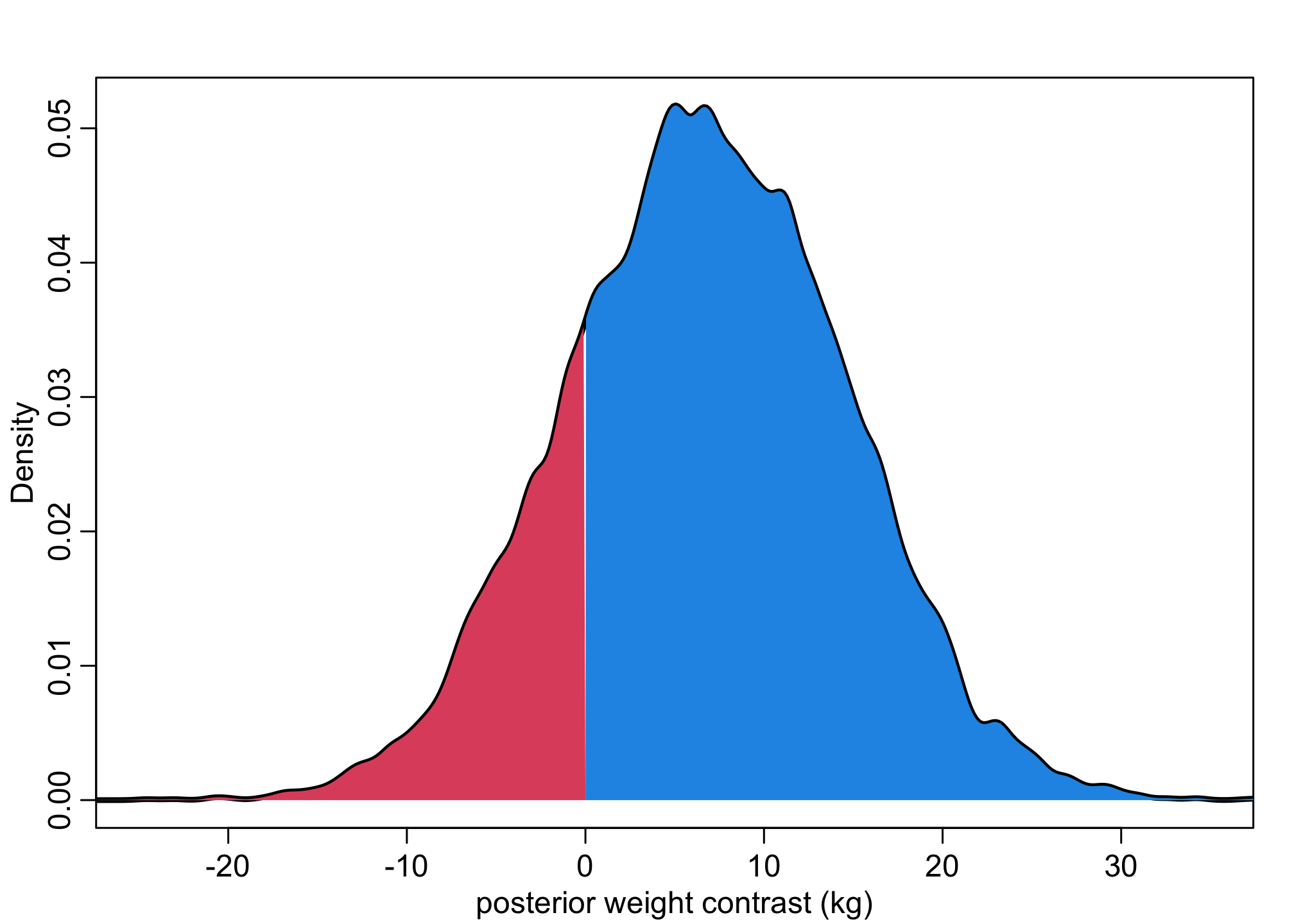
Thought question: Why was including height into the regression enabling estimation of the direct effect of sex on weight? Why was removing height enabling a total effect of sex on weight?

Full Luxury Bayes (Optional)

This part is covered in Lecture 4 briefly – note, we won’t go in depth so only review this example if you want to understand more.

In this setup, we’ll run height and weight simultaneously.

# full system as SCM
dat <- list(
    W = d$weight,
    H = d$height,
    Hbar = mean(d$height),
    S = d$male + 1 ) # S=1 female, S=2 male

m_SHW_full <- quap(
    alist(

        # weight
        W ~ dnorm(mu,sigma),
        mu <- a[S] + b[S]*(H-Hbar),
        a[S] ~ dnorm(60,10),
        b[S] ~ dlnorm(0,1),
        sigma ~ dunif(0,10),

        # height
        H ~ dnorm(nu,tau),
        nu <- h[S],
        h[S] ~ dnorm(160,10),
        tau ~ dunif(0,10)

    ), data=dat )

We’ll simulate 1000 synthetic women in order. We focus on height first since it’s a function of weight. Then simulate weights by using the simulation heights. Then repeat for 1000 synthetic men in the similar order.

# compute total causal effect of S on W
post <- extract.samples(m_SHW_full)
Hbar <- dat$Hbar
n <- 1e4

with( post , {
# simulate W for S=1
  H_S1 <- rnorm(n, h[,1] , tau )
  W_S1 <- rnorm(n, a[,1] + b[,1]*(H_S1-Hbar) , sigma)
# simulate W for S=2
  H_S2 <- rnorm(n, h[,2] , tau)
  W_S2 <- rnorm(n, a[,2] + b[,2]*(H_S2-Hbar) , sigma)
# compute contrast (do operator); should hold results from intervening in sex
  W_do_S <<- W_S2 - W_S1
# <<- (scoping assignment)
#https://stackoverflow.com/questions/2628621/how-do-you-use-scoping-assignment-in-r
})

dens( W_do_S , xlim=c(-25,35) , lwd=3 , col=1 , xlab="posterior weight contrast (kg)" )

Wdens <- density(W_do_S,adj=0.5)
polygon(c(Wdens$x[Wdens$x>0], max(Wdens$x), 0), c(Wdens$y[Wdens$x>0], 0, 0), col = 4, border = NA )
polygon(c(Wdens$x[Wdens$x<0], 0, min(Wdens$x)), c(Wdens$y[Wdens$x<0], 0, 0), col = 2, border = NA )

# automated way
HWsim <- sim(m_SHW_full,
             data=list(S=c(1,2)),
             vars=c("H","W"))
W_do_S_auto <- HWsim$W[,2] - HWsim$W[,1]

Package versions

sessionInfo()

## R version 4.1.1 (2021-08-10)
## Platform: aarch64-apple-darwin20 (64-bit)
## Running under: macOS Monterey 12.1
## 
## Matrix products: default
## BLAS:   /Library/Frameworks/R.framework/Versions/4.1-arm64/Resources/lib/libRblas.0.dylib
## LAPACK: /Library/Frameworks/R.framework/Versions/4.1-arm64/Resources/lib/libRlapack.dylib
## 
## locale:
## [1] en_US.UTF-8/en_US.UTF-8/en_US.UTF-8/C/en_US.UTF-8/en_US.UTF-8
## 
## attached base packages:
## [1] parallel  stats     graphics  grDevices datasets  utils     methods  
## [8] base     
## 
## other attached packages:
## [1] dagitty_0.3-1        rethinking_2.21      cmdstanr_0.4.0.9001 
## [4] rstan_2.21.3         ggplot2_3.3.5        StanHeaders_2.21.0-7
## 
## loaded via a namespace (and not attached):
##  [1] sass_0.4.0           jsonlite_1.7.2       bslib_0.3.1         
##  [4] RcppParallel_5.1.4   assertthat_0.2.1     posterior_1.1.0     
##  [7] distributional_0.2.2 highr_0.9            stats4_4.1.1        
## [10] tensorA_0.36.2       renv_0.14.0          yaml_2.2.1          
## [13] pillar_1.6.4         backports_1.4.1      lattice_0.20-44     
## [16] glue_1.6.0           uuid_1.0-3           digest_0.6.29       
## [19] checkmate_2.0.0      colorspace_2.0-2     htmltools_0.5.2     
## [22] pkgconfig_2.0.3      bookdown_0.24        purrr_0.3.4         
## [25] mvtnorm_1.1-3        scales_1.1.1         processx_3.5.2      
## [28] tibble_3.1.6         generics_0.1.1       farver_2.1.0        
## [31] ellipsis_0.3.2       withr_2.4.3          cli_3.1.0           
## [34] mime_0.12            magrittr_2.0.1       crayon_1.4.2        
## [37] evaluate_0.14        ps_1.6.0             fs_1.5.0            
## [40] fansi_0.5.0          MASS_7.3-54          pkgbuild_1.3.1      
## [43] blogdown_1.5         tools_4.1.1          loo_2.4.1           
## [46] prettyunits_1.1.1    lifecycle_1.0.1      matrixStats_0.61.0  
## [49] stringr_1.4.0        V8_3.6.0             munsell_0.5.0       
## [52] callr_3.7.0          compiler_4.1.1       jquerylib_0.1.4     
## [55] rlang_0.4.12         grid_4.1.1           rstudioapi_0.13     
## [58] base64enc_0.1-3      rmarkdown_2.11       boot_1.3-28         
## [61] xaringanExtra_0.5.5  gtable_0.3.0         codetools_0.2-18    
## [64] curl_4.3.2           inline_0.3.19        abind_1.4-5         
## [67] DBI_1.1.1            R6_2.5.1             gridExtra_2.3       
## [70] lubridate_1.8.0      knitr_1.36           dplyr_1.0.7         
## [73] fastmap_1.1.0        utf8_1.2.2           downloadthis_0.2.1  
## [76] bsplus_0.1.3         shape_1.4.6          stringi_1.7.6       
## [79] Rcpp_1.0.7           vctrs_0.3.8          tidyselect_1.1.1    
## [82] xfun_0.28            coda_0.19-4

Last updated on Feb 13, 2022