Class 3

Introduction
For this class, we’ll review code examples found in Chapter 4.
This assumes that you have already installed the rethinking package.
If you need help, be sure to remember the references in the Resources:
Chapter 4
Drawing the Owl

1. Question or estimand
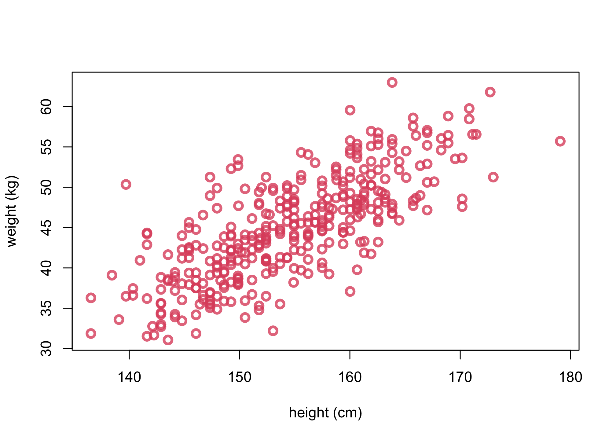
Objective: Describe the association between Adult weight and height
library(rethinking)
data(Howell1)
d <- Howell1[Howell1$age>=18,]

plot(d$height, d$weight, col = 2,  xlab = "height (cm)", ylab = "weight (kg)",  lwd=3)

2. Scientific model
Weight is a function of height.
library(dagitty)

g <- dagitty('dag {
    H [pos="0,1"]
    W [pos="1,1"]

    H -> W
}')
plot(g)
3. Statistical model
Generative Model
Let’s consider the Generative Model (H -> W) from the lecture:
\(W_i \sim Normal(\mu_i,\sigma)\)\(\mu_i = \alpha + \beta H_i\)
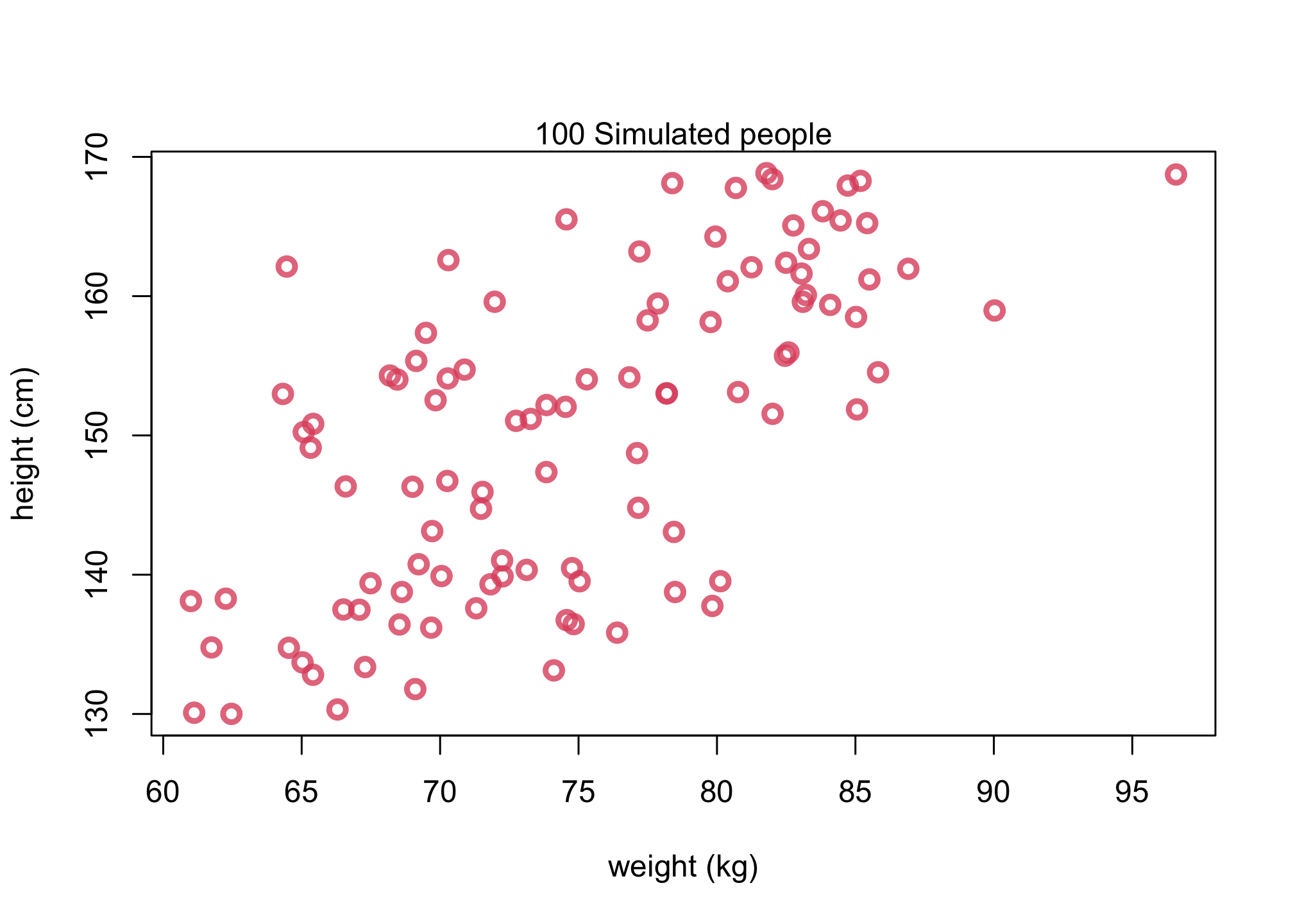
Let’s now conduct a prior predictive simulation to simulate “synthetic individuals.”
set.seed(17)
# forward simulation as we choose these parameters
alpha <- 0 # implies zero height => zero weight
beta <- 0.5
sigma <- 5
n_individuals <- 100

H <- runif(n_individuals,130,170) # heights, uniform between 130 - 170 cm
mu <- alpha + beta*H
W <- rnorm(n_individuals,mu,sigma) # sample from Normal
col2 <- col.alpha(2,0.8)
plot(W,H,  col=col2, lwd=3,
     cex=1.2,  xlab = "weight (kg)", ylab = "height (cm)")
mtext( "100 Simulated people" )
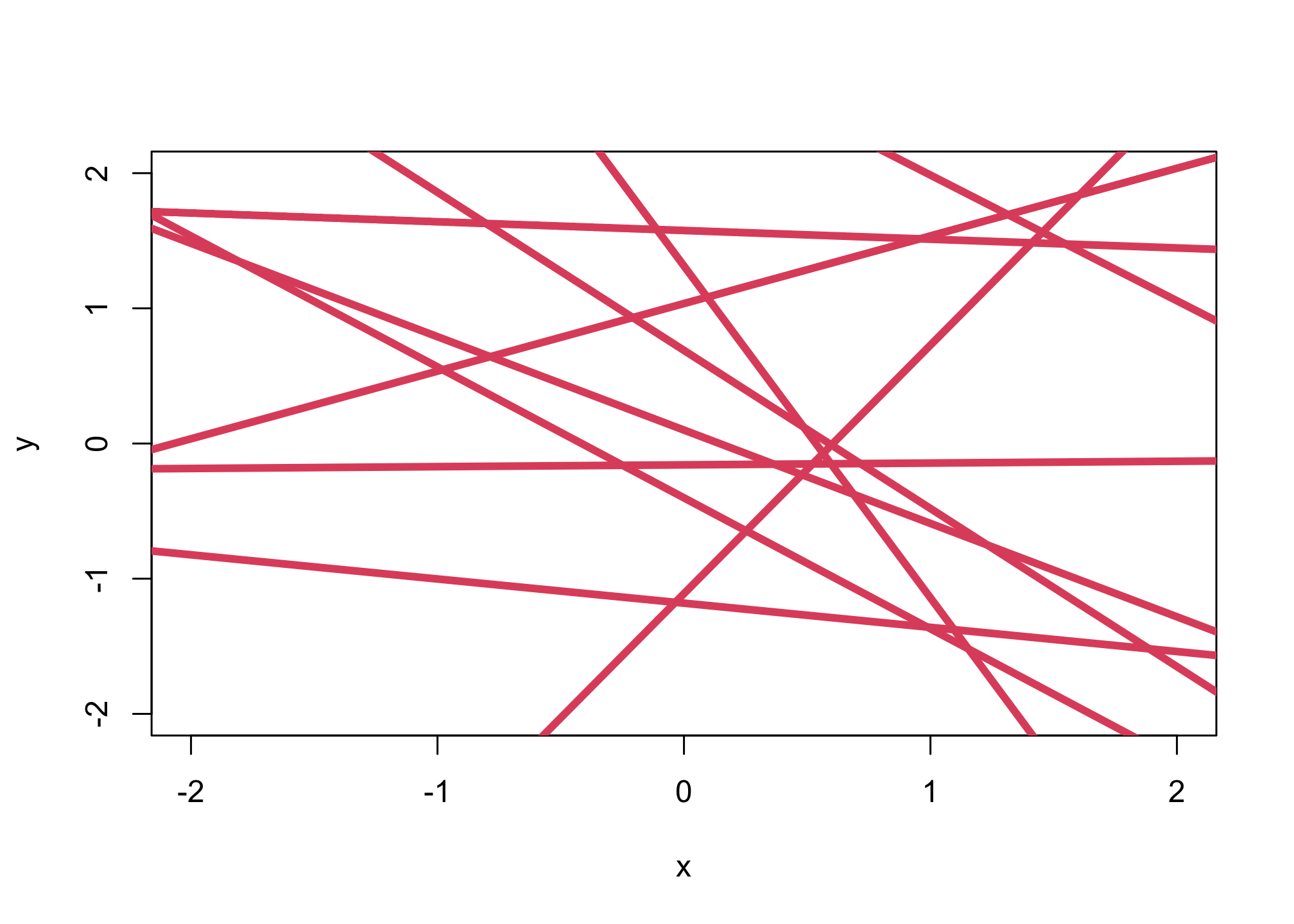
Sampling the prior distribution
n_samples <- 10

alpha <- rnorm(n_samples,0,1)
beta <- rnorm(n_samples,0,1)

plot(NULL,xlim=c(-2,2),ylim=c(-2,2),xlab="x",ylab="y")
for (i in 1:n_samples){
  abline(alpha[i],beta[i],lwd=4,col=2)
}
3. Statistical model for H->W
n <- 10
alpha <- rnorm(n,60,10)
beta <- rnorm(n,0,10)

Hbar <- 150
Hseq <- seq(from=130,to=170,len=30)
plot(NULL, xlim=c(130,170), ylim=c(10,100),
     xlab="height (cm)", ylab="weight (kg)")

for (i in 1:n){
  lines(Hseq, alpha[i] + beta[i]*(Hseq-Hbar),lwd=3,col=2)
}
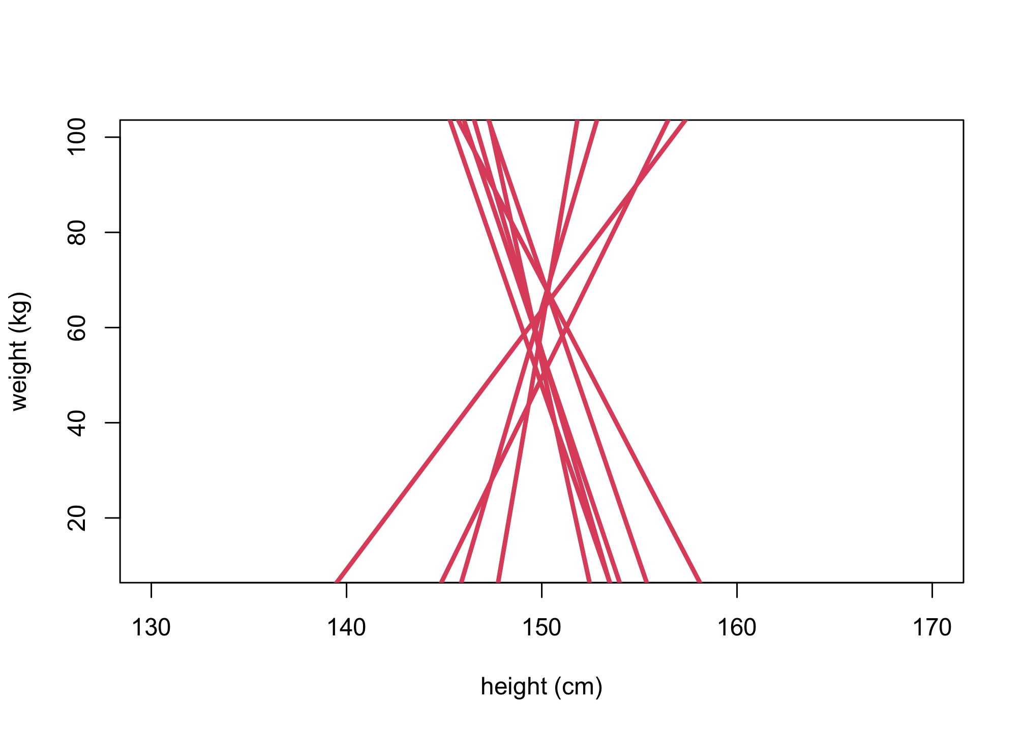
Is this a good prior to be used? Why or why not are they interpretable?
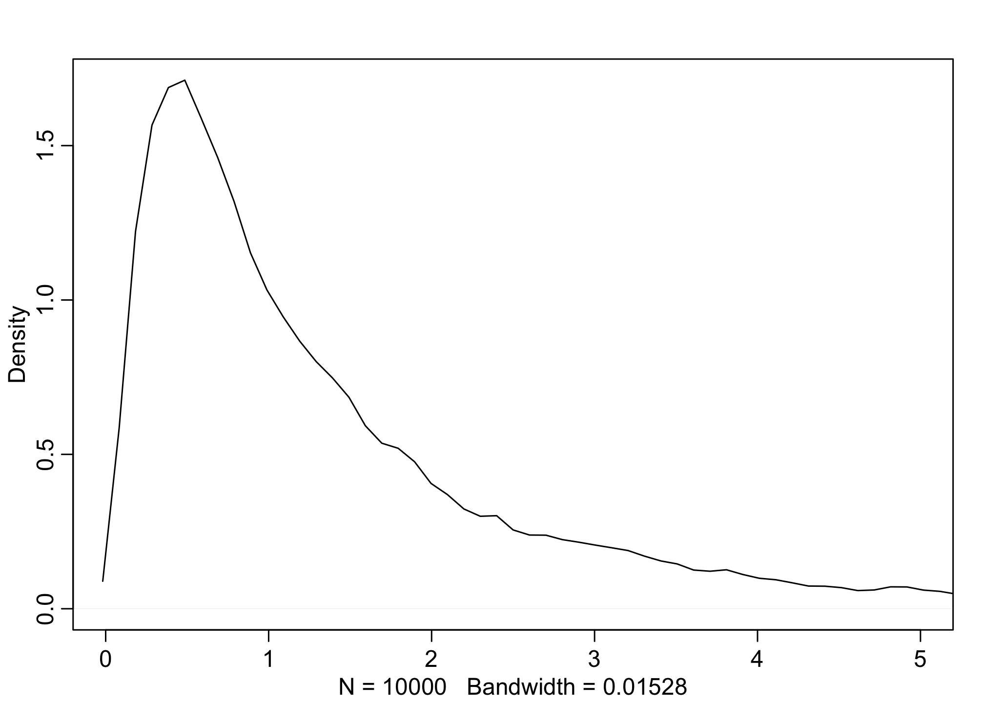
Remember, a lognormal distribution is a distribution that if you take the logarithm of the values, then all of it’s values would be normal.
# simulated lognormal
b <- rlnorm(1e4, 0, 1) #4.40
dens(b, xlim=c(0,5), adj=0.1)
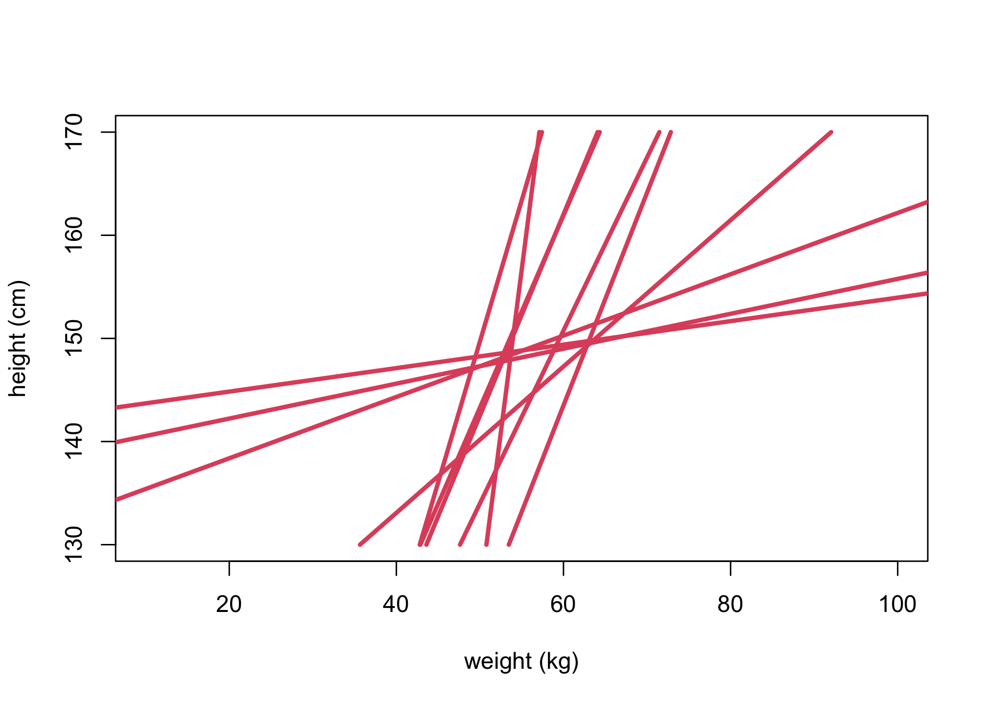
Let’s do a predictive simulation now using the Log-Normal prior.
set.seed(2971)
n <- 10
a <- rnorm( n , 60 , 5 )
b <- rlnorm( n , 0 , 1 )

plot(NULL, ylim=c(130,170), xlim=c(10,100),
     ylab="height (cm)", xlab="weight (kg)")

for (i in 1:n){
  lines(a[i] + b[i]*(Hseq-Hbar),Hseq, lwd=3,col=2)
}
\(W_i \sim Normal(\mu_i,\sigma)\)\(\mu_i = \alpha + \beta(H_i - \overline{H})\)\(\alpha \sim Normal(178,20)\)\(\beta \sim LogNormal(0,1)\)\(\sigma \sim Uniform(0,50)\)
# define the average weight, x-bar
xbar <- mean(d$weight)

# fit model
m4.3 <- quap(
    alist(
        height ~ dnorm( mu , sigma ) ,
        mu <- a + b*( weight - xbar ) ,
        a ~ dnorm( 178 , 20 ) ,
        b ~ dlnorm( 0 , 1 ) ,
        sigma ~ dunif( 0 , 50 )
    ) , data=d )

## R code 4.44
precis( m4.3 )
##              mean         sd        5.5%       94.5%
## a     154.6013728 0.27030783 154.1693687 155.0333770
## b       0.9032803 0.04192366   0.8362782   0.9702824
## sigma   5.0718842 0.19115509   4.7663814   5.3773869
The first row gives the quadratic approximation for α, the second the approximation for β, and the third approximation for σ.
Let’s focus on b (β). Since β is a slope, the value 0.90 can be read as a person 1 kg heavier is expected to be 0.90 cm taller. 89% of the posterior probability lies between 0.84 and 0.97. That suggests that β values close to zero or greatly above one are highly incompatible with these data and this model. It is most certainly not evidence that the relationship between weight and height is linear, because the model only considered lines. It just says that, if you are committed to a line, then lines with a slope around 0.9 are plausible ones.
## R code 4.45
round( vcov( m4.3 ) , 3 )
##           a     b sigma
## a     0.073 0.000 0.000
## b     0.000 0.002 0.000
## sigma 0.000 0.000 0.037
# shows both the marginal posteriors and the covariance.
pairs(m4.3)
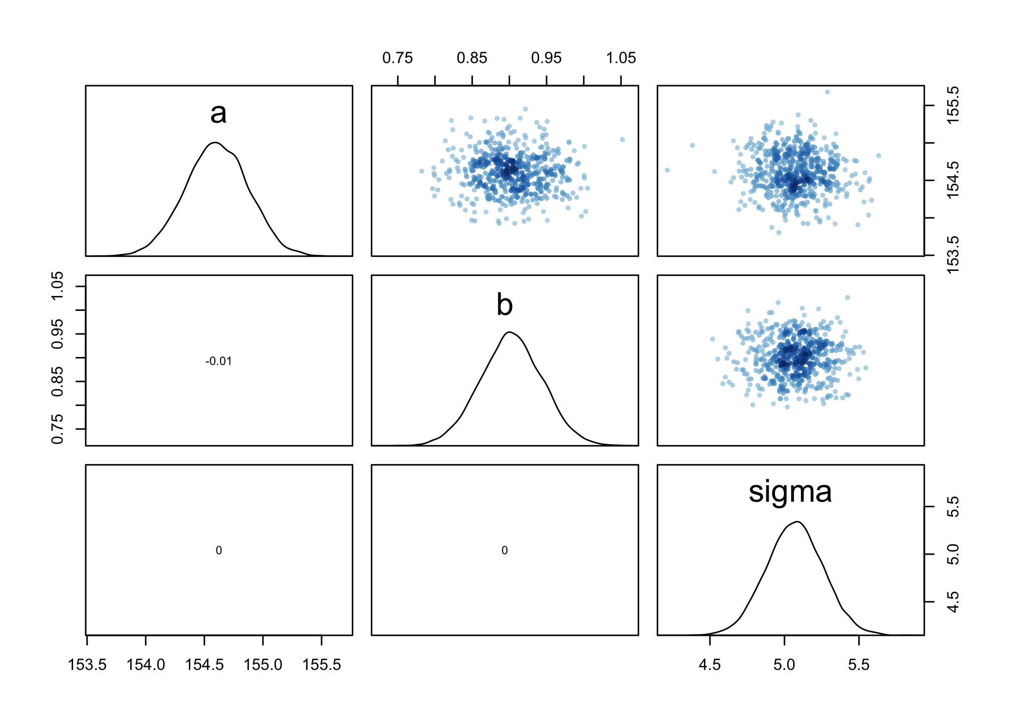
There is little covariation among the parameters in this case. The lack of covariance among the parameters results from centering.
As an exercise, consider rerunning the regression above without centering and compare the covariation.
4. Validate model
We’ll use a simulation-based validation.
We’ll first validate with a simulation (aka fake data).
\(W_i \sim Normal(\mu_i,\sigma)\)\(\mu_i = \alpha + \beta(H_i - \overline{H})\)\(\alpha \sim Normal(60,10)\)\(\beta \sim LogNormal(0,1)\)\(\sigma \sim Uniform(0,10)\)
alpha <- 70
beta <- 0.5
sigma <- 5
n_individuals <- 100

# simulation
H <- runif(n_individuals,130,170)
mu <- alpha + beta*(H-mean(H))
W <- rnorm(n_individuals,mu,sigma)

dat <- list(H=H,W=W,Hbar=mean(H))

m_validate <- quap(
    alist(
        W ~ dnorm( mu , sigma ) ,
        mu <- a + b*( H - Hbar ),
        a ~ dnorm( 60 , 10 ) ,
        b ~ dlnorm( 0 , 1 ) ,
        sigma ~ dunif( 0 , 10 )
    ) , data=dat )

precis(m_validate)
##             mean         sd       5.5%      94.5%
## a     69.9483419 0.46670241 69.2024614 70.6942225
## b      0.5139771 0.03867635  0.4521648  0.5757894
## sigma  4.6720149 0.33036867  4.1440220  5.2000079
Let’s now run it with real data.
dat <- list(W = d$weight, H = d$height, Hbar = mean(d$height))

m_adults <- quap(
    alist(
        W ~ dnorm( mu , sigma ) ,
        mu <- a + b*( H - Hbar ),
        a ~ dnorm( 60 , 10 ) ,
        b ~ dlnorm( 0 , 1 ) ,
        sigma ~ dunif( 0 , 10 )
    ) , data=dat )

precis(m_adults)
##             mean         sd       5.5%      94.5%
## a     44.9981241 0.22538919 44.6379087 45.3583396
## b      0.6286797 0.02914554  0.5820995  0.6752599
## sigma  4.2297367 0.15941778  3.9749563  4.4845171
First Law of Statistical Interpretation: The parameters are not independent of one another and cannot always be independently interpreted.
Instead, draw (push out) posterior predictions and describe/interpret them.
post <- extract.samples(m_adults)
head(post)
##          a         b    sigma
## 1 44.80946 0.6584680 4.121912
## 2 45.56093 0.6486405 4.262163
## 3 45.07283 0.6567565 4.228691
## 4 44.98621 0.5895380 4.215656
## 5 44.99444 0.6983031 3.891291
## 6 45.05029 0.5888397 4.196087
1. Plot the sample
# 4.4.3
col2 <- col.alpha(2,0.8)
plot(d$height, d$weight, col=col2, lwd=3,
     cex=1.2, xlab="height (cm)", ylab="weight (kg)")
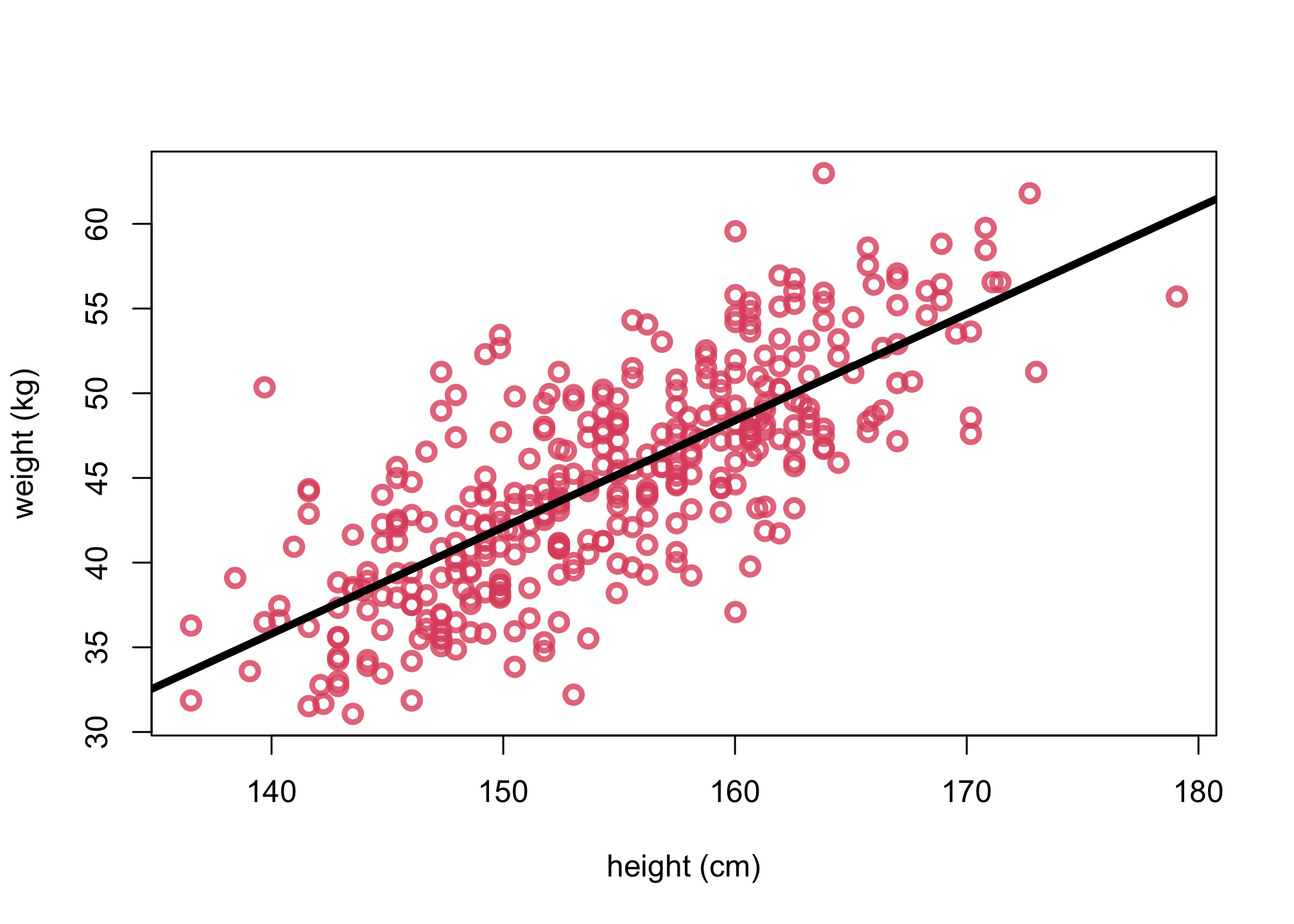
2. Plot the posterior mean
# get posterior mean via link function
xseq <- seq(from=130,to=190,len=50)
mu <- link(m_adults,data=list( H=xseq,Hbar=mean(d$height)))
mu.mean <- apply( mu , 2 , mean )

# plot same with lines for mu.mean
plot(d$height, d$weight, col=col2, lwd=3,
     cex=1.2, xlab="height (cm)", ylab="weight (kg)")
lines(xseq, mu.mean, lwd=4)
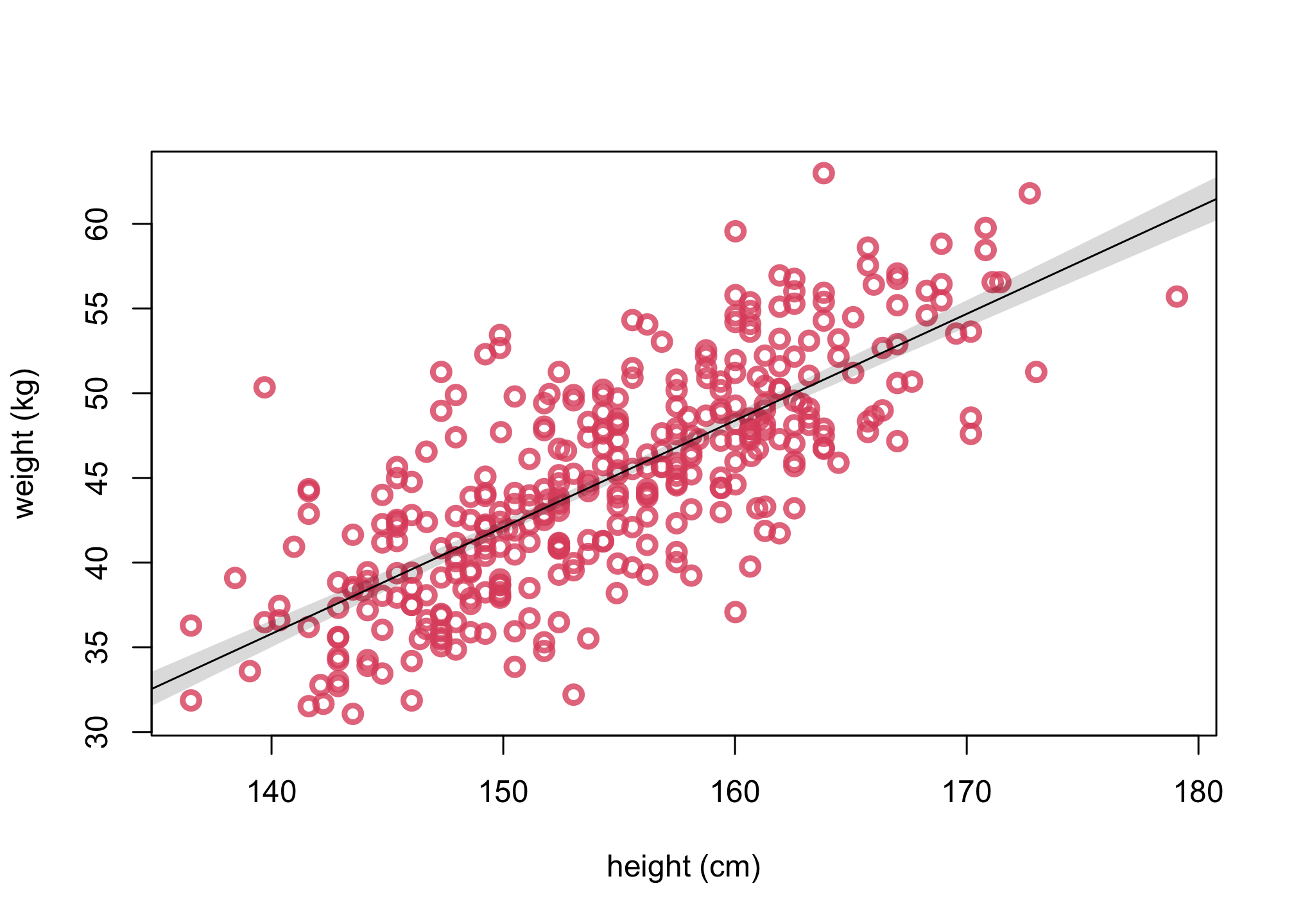
3. Plot uncertainty of the mean
# get PI for mu
mu.PI <- apply( mu , 2 , PI , prob=0.89 )

# replot same as 2
plot(d$height, d$weight, col=col2 , lwd=3,
     cex=1.2, xlab="height (cm)", ylab="weight (kg)")
lines( xseq , mu.mean )
# add plot a shaded region for 89% PI
shade( mu.PI , xseq )
#alternative way to plot uncertainty of the mean
#for ( i in 1:100 )
#    lines( xseq , mu[i,] , pch=16, col=col.alpha(rangi2,0.1) )
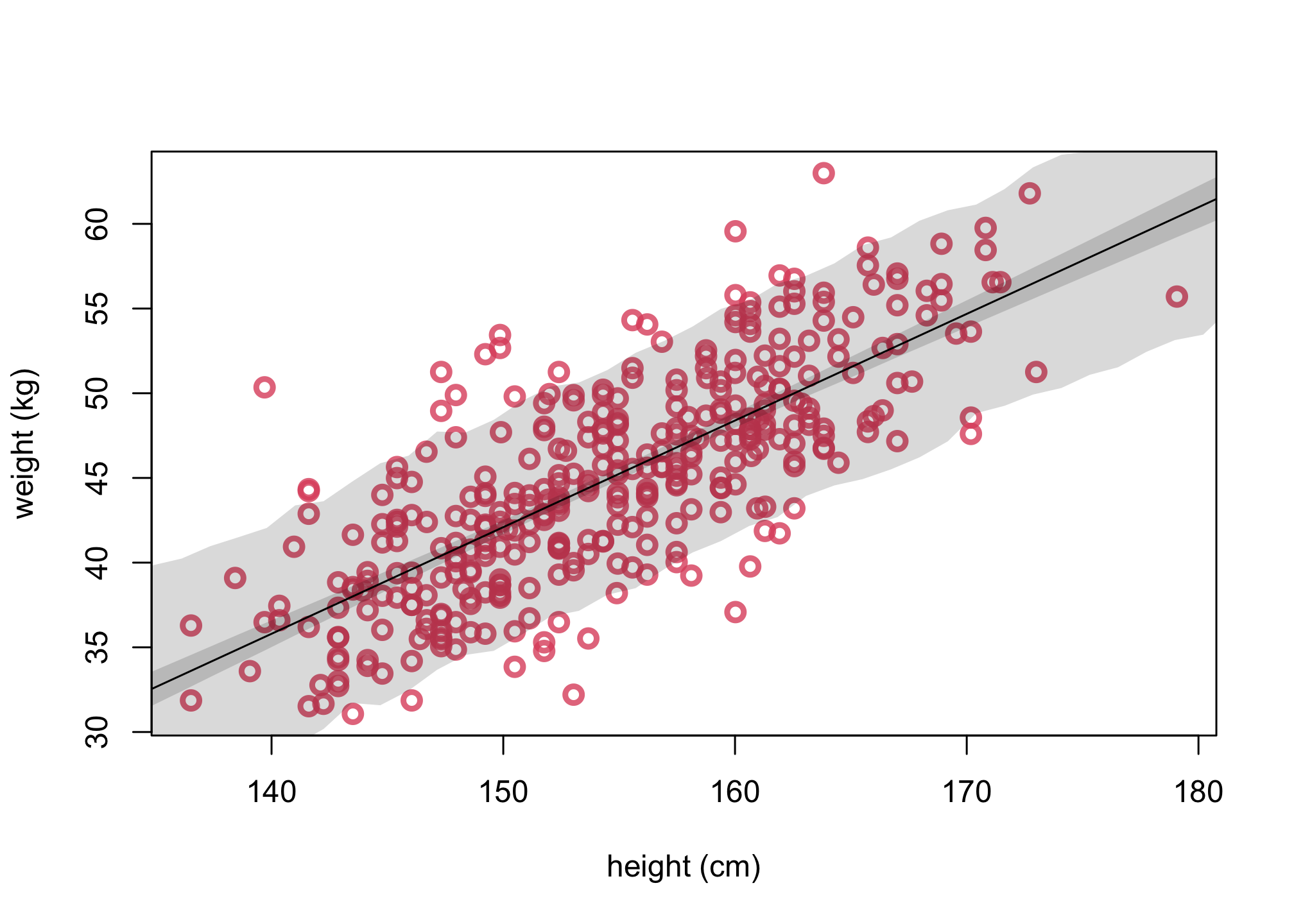
4. Plot uncertainty of predictions
# simulate hypothetical adjusts given xseq
sim.height <- sim( m_adults , data=list(H=xseq,Hbar=mean(d$height)))
height.PI <- apply( sim.height , 2 , PI , prob=0.89 )

# replot 3
plot( d$height,d$weight, col=col2 , lwd=3,
     cex=1.2, xlab="height (cm)", ylab="weight (kg)")
lines( xseq, mu.mean)
shade( mu.PI , xseq )

# add in PI region for simulated heights
shade( height.PI , xseq )
Example
Let’s say we want to simulate using the m_adults model four individuals, each with heights 140, 150, 170, and 190.
Calculate the simulated mean weights and 89% percentile intervals for these four individuals.
set.seed(100)
sample_heights = c(135,150,170,190)

simul_weights <- sim( m_adults , data=list(H=sample_heights,Hbar=mean(d$height)))

# simulated means
mean_weights = apply( simul_weights , 2 , mean )
mean_weights
## [1] 32.52395 42.15084 54.84502 67.30787
# simulated PI's
pi_weights = apply( simul_weights , 2 , PI , prob=0.89 )
pi_weights
##         [,1]     [,2]     [,3]     [,4]
## 5%  25.86437 35.55815 48.21862 60.84940
## 94% 39.40483 48.65104 61.45551 73.87156
data.frame(
  sample_heights = sample_heights,
  simulated_mean = mean_weights,
  low_pi = pi_weights[1,],
  high_pi = pi_weights[2,]
)
##   sample_heights simulated_mean   low_pi  high_pi
## 1            135       32.52395 25.86437 39.40483
## 2            150       42.15084 35.55815 48.65104
## 3            170       54.84502 48.21862 61.45551
## 4            190       67.30787 60.84940 73.87156
Package versions
sessionInfo()
## R version 4.1.1 (2021-08-10)
## Platform: aarch64-apple-darwin20 (64-bit)
## Running under: macOS Monterey 12.1
##
## Matrix products: default
## BLAS:   /Library/Frameworks/R.framework/Versions/4.1-arm64/Resources/lib/libRblas.0.dylib
## LAPACK: /Library/Frameworks/R.framework/Versions/4.1-arm64/Resources/lib/libRlapack.dylib
##
## locale:
## [1] en_US.UTF-8/en_US.UTF-8/en_US.UTF-8/C/en_US.UTF-8/en_US.UTF-8
##
## attached base packages:
## [1] parallel  stats     graphics  grDevices datasets  utils     methods
## [8] base
##
## other attached packages:
## [1] dagitty_0.3-1        rethinking_2.21      cmdstanr_0.4.0.9001
## [4] rstan_2.21.3         ggplot2_3.3.5        StanHeaders_2.21.0-7
##
## loaded via a namespace (and not attached):
##  [1] sass_0.4.0           jsonlite_1.7.2       bslib_0.3.1
##  [4] RcppParallel_5.1.4   assertthat_0.2.1     posterior_1.1.0
##  [7] distributional_0.2.2 highr_0.9            stats4_4.1.1
## [10] tensorA_0.36.2       renv_0.14.0          yaml_2.2.1
## [13] pillar_1.6.4         backports_1.4.1      lattice_0.20-44
## [16] glue_1.6.0           uuid_1.0-3           digest_0.6.29
## [19] checkmate_2.0.0      colorspace_2.0-2     htmltools_0.5.2
## [22] pkgconfig_2.0.3      bookdown_0.24        purrr_0.3.4
## [25] mvtnorm_1.1-3        scales_1.1.1         processx_3.5.2
## [28] tibble_3.1.6         generics_0.1.1       farver_2.1.0
## [31] ellipsis_0.3.2       withr_2.4.3          cli_3.1.0
## [34] mime_0.12            magrittr_2.0.1       crayon_1.4.2
## [37] evaluate_0.14        ps_1.6.0             fs_1.5.0
## [40] fansi_0.5.0          MASS_7.3-54          pkgbuild_1.3.1
## [43] blogdown_1.5         tools_4.1.1          loo_2.4.1
## [46] prettyunits_1.1.1    lifecycle_1.0.1      matrixStats_0.61.0
## [49] stringr_1.4.0        V8_3.6.0             munsell_0.5.0
## [52] callr_3.7.0          compiler_4.1.1       jquerylib_0.1.4
## [55] rlang_0.4.12         grid_4.1.1           rstudioapi_0.13
## [58] base64enc_0.1-3      rmarkdown_2.11       boot_1.3-28
## [61] xaringanExtra_0.5.5  gtable_0.3.0         codetools_0.2-18
## [64] curl_4.3.2           inline_0.3.19        abind_1.4-5
## [67] DBI_1.1.1            R6_2.5.1             gridExtra_2.3
## [70] lubridate_1.8.0      knitr_1.36           dplyr_1.0.7
## [73] fastmap_1.1.0        utf8_1.2.2           downloadthis_0.2.1
## [76] bsplus_0.1.3         KernSmooth_2.23-20   shape_1.4.6
## [79] stringi_1.7.6        Rcpp_1.0.7           vctrs_0.3.8
## [82] tidyselect_1.1.1     xfun_0.28            coda_0.19-4