Class 2

Introduction
For this class, we’ll review code examples found in Chapter 2.
This assumes that you have already installed the rethinking package.
If you need help, be sure to remember the references in the Resources:
Chapter 2
Bayesian Updating: Grid Approximation
Let’s assume we have the table in 2.1
## R code 2.1
ways <- c( 0 , 3 , 8 , 9 , 0 )
ways/sum(ways)
## [1] 0.00 0.15 0.40 0.45 0.00
Let’s compute the likelihood of six W’s in nine tosses (assuming a 50% probability):
## R code 2.2
dbinom( 6 , size=9 , prob=0.5 )
## [1] 0.1640625
We can see it’s 16.4%.
Be sure to examine the dbinom function by typing in ?dbinom and exploring the documentation. We’ll use this function a lot in this class.
Next, let’s define a grid. This is required when we are using Grid Approximation for our Bayesian calculations (i.e., to estimate the posterior).
## R code 2.3
# define grid
p_grid <- seq( from=0 , to=1 , length.out=20 )

p_grid
##  [1] 0.00000000 0.05263158 0.10526316 0.15789474 0.21052632 0.26315789
##  [7] 0.31578947 0.36842105 0.42105263 0.47368421 0.52631579 0.57894737
## [13] 0.63157895 0.68421053 0.73684211 0.78947368 0.84210526 0.89473684
## [19] 0.94736842 1.00000000
Notice that this function creates a vector with length 20 and that ranges from 0 to 1. Note as well that each vector element is evenly spaced in increments of (to - from)/(length.out - 1).
Think about the trade-off between having a smaller or larger length.out.
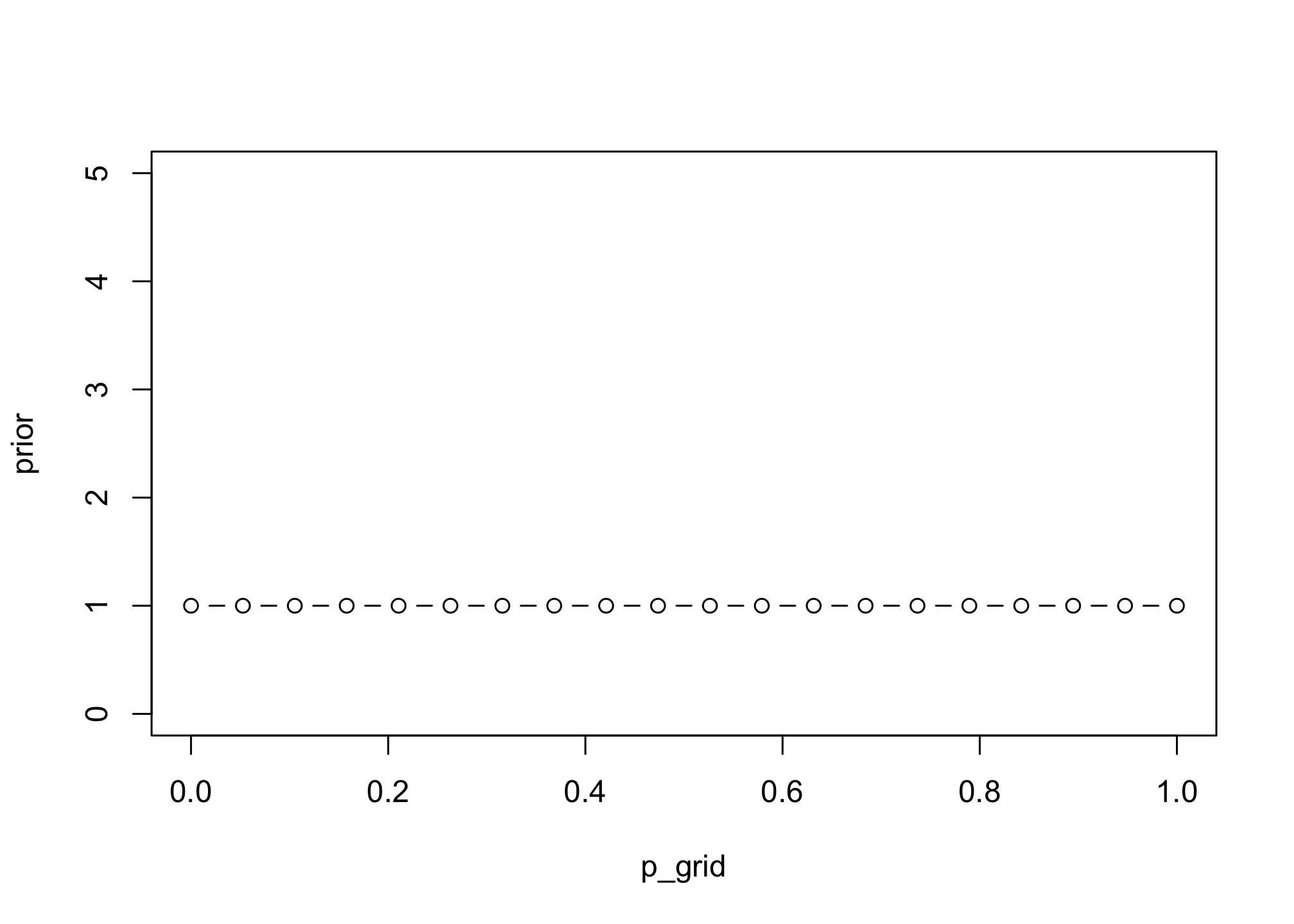
Next, let’s define our prior. We’ll assume a “flat” prior.
# define prior
prior <- rep( 1 , 20 )

plot(p_grid, prior, type="b", ylim=c(0,5))
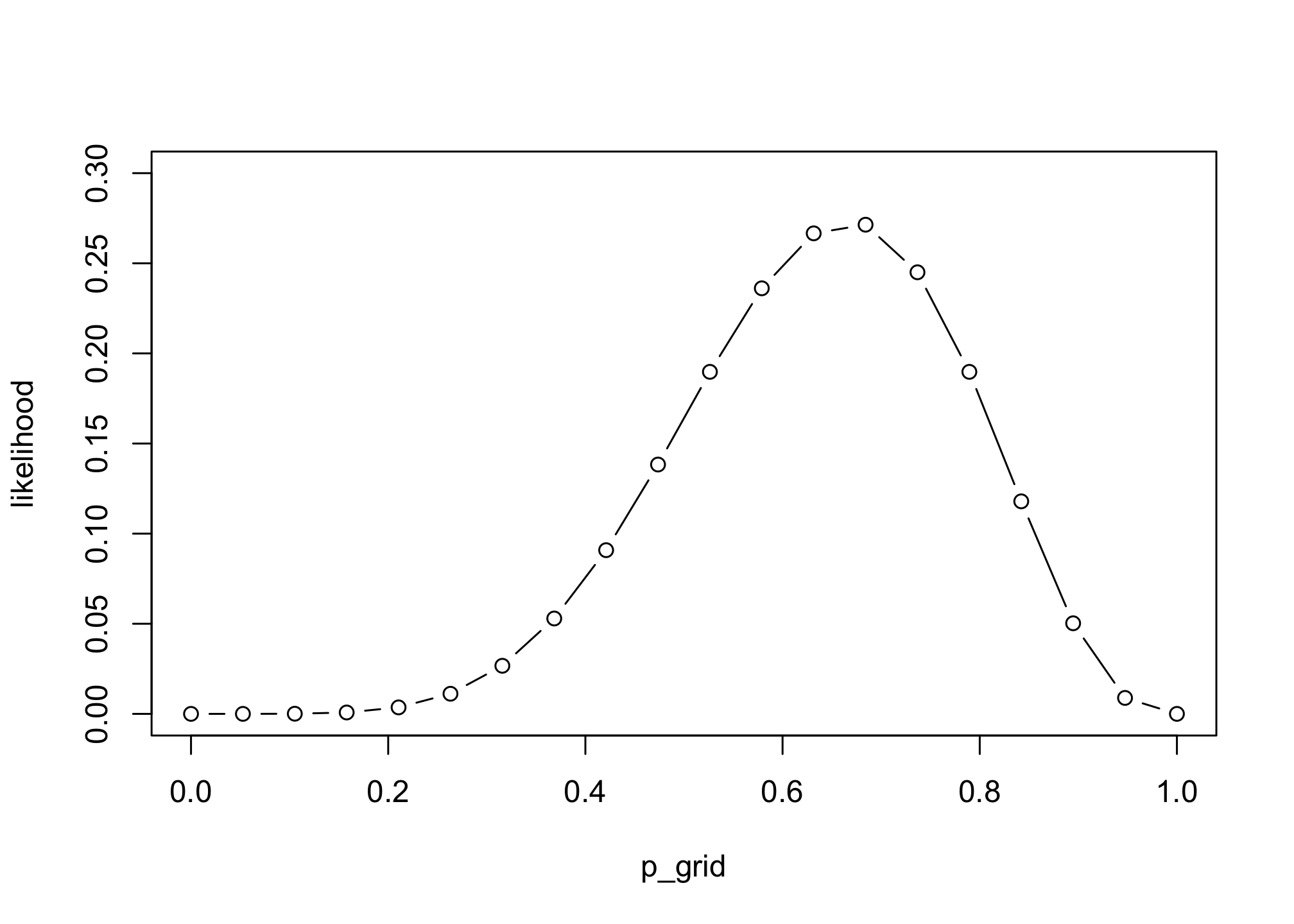
# compute likelihood at each value in grid
likelihood <- dbinom( 6 , size=9 , prob=p_grid )

plot(p_grid, likelihood, type="b", ylim=c(0,0.3))
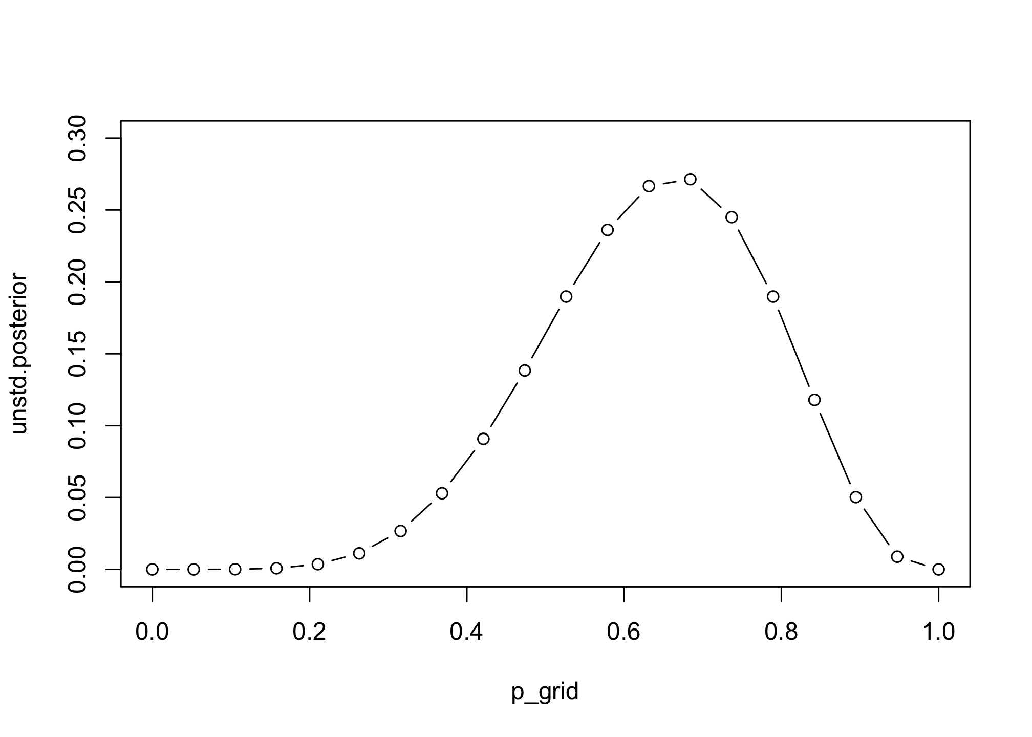
# compute product of likelihood and prior
unstd.posterior <- likelihood * prior

plot(p_grid, unstd.posterior, type="b", ylim=c(0,0.3))
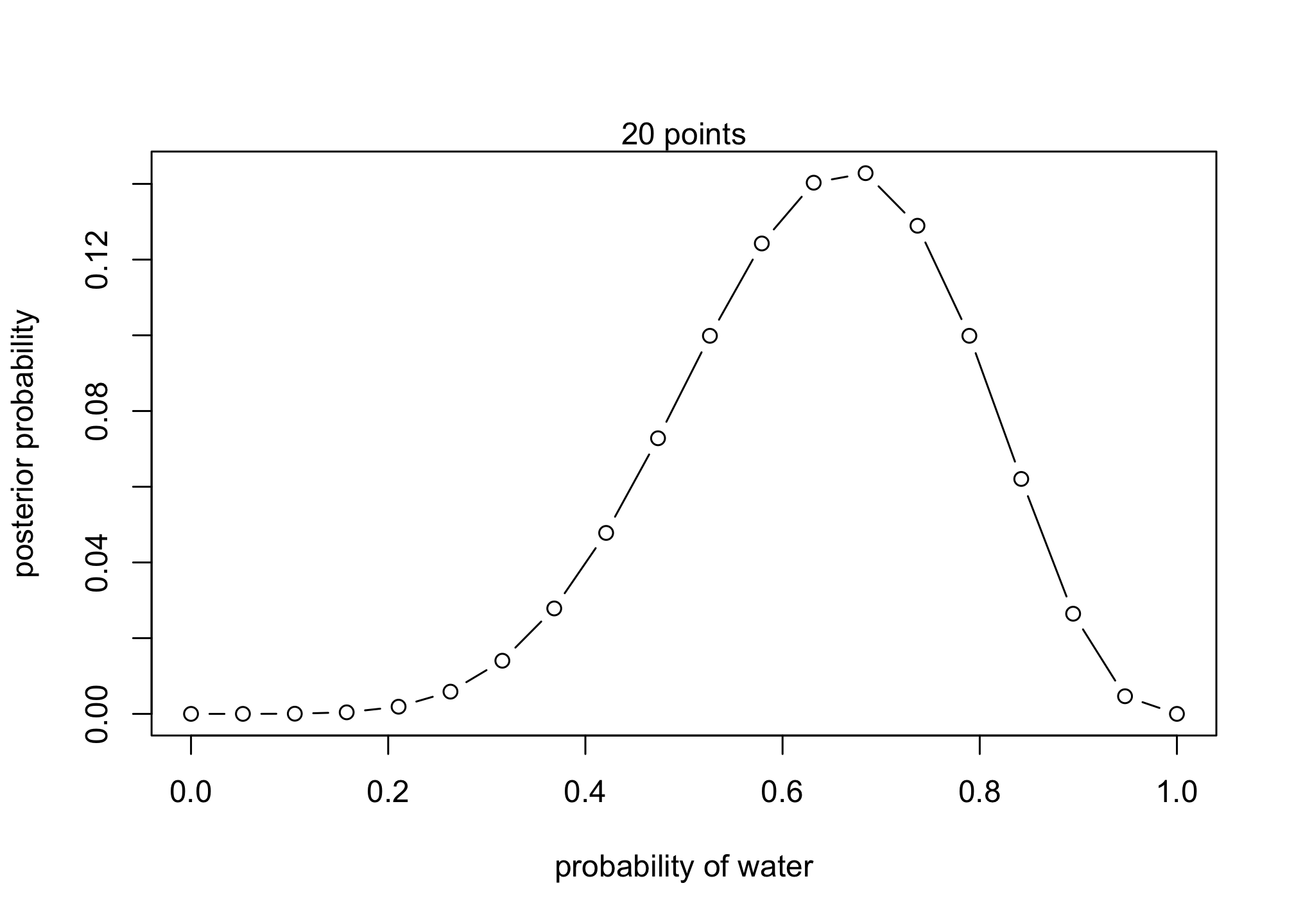
# standardize the posterior, so it sums to 1
posterior <- unstd.posterior / sum(unstd.posterior)
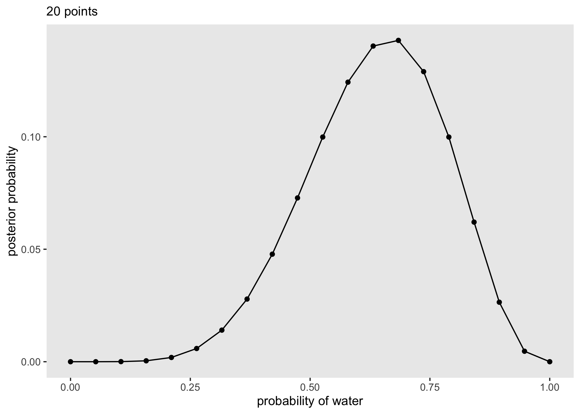
## R code 2.4
plot( p_grid , posterior , type="b" ,
xlab="probability of water" , ylab="posterior probability" )
mtext( "20 points" )
Practice: What happens if we alter the priors? What will be the new posteriors?
Assume 6 W’s and 3 L’s (9 tosses). Plot the posterior and compare them to using a uniform prior.
# prior 1
prior <- ifelse( p_grid < 0.5 , 0 , 1 )
# prior 2
prior <- exp( -5*abs( p_grid - 0.5 ) )
Bayesian Updating: Quadratic Approximation
We can also use quadratic approximation, which is discussed on page 42 of Chapter2. We’ll use quadratic approximation approach over the next few weeks before moving to MCMC methods via Stan.
## R code 2.6
library(rethinking)
globe.qa <- quap(
    alist(
        W ~ dbinom( W+L ,p) ,  # binomial likelihood
        p ~ dunif(0,1)     # uniform prior
    ) ,
    data=list(W=6,L=3) )

globe.qa
##
## Quadratic approximate posterior distribution
##
## Formula:
## W ~ dbinom(W + L, p)
## p ~ dunif(0, 1)
##
## Posterior means:
##         p
## 0.6666663
##
## Log-likelihood: -1.3
We can also use the precis function to summarize parameter estimates. I recommend running ?precis to look up parameters associated with this function.
# display summary of quadratic approximation
precis( globe.qa )
##        mean        sd      5.5%     94.5%
## p 0.6666663 0.1571339 0.4155361 0.9177966
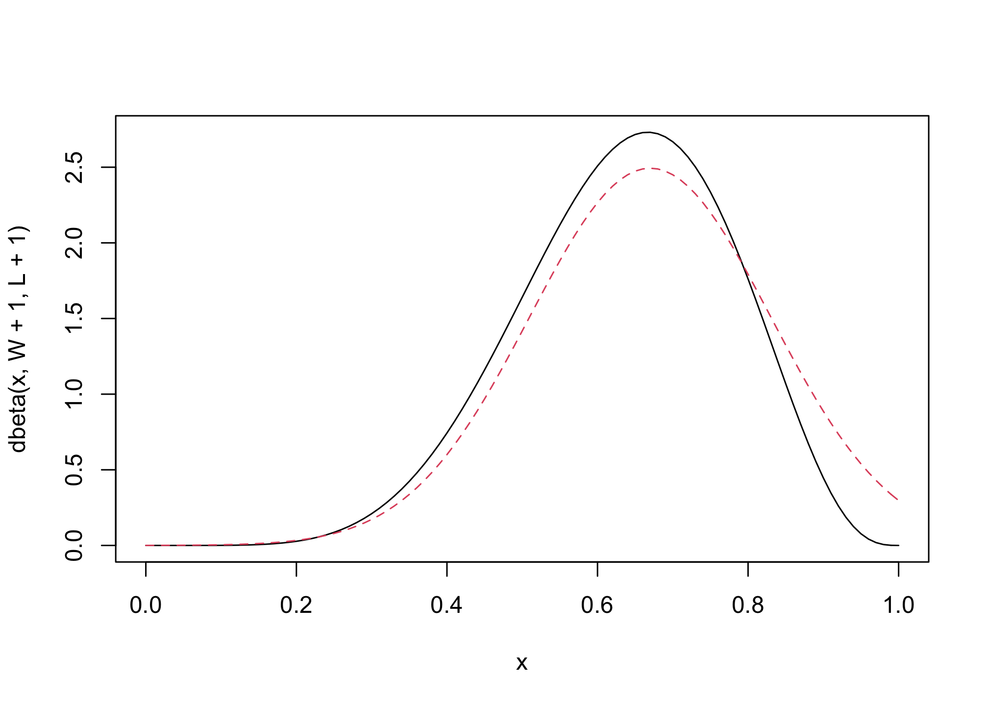
How does grid approximation compare to analytical posterior calculation?
## R code 2.7
# analytical calculation
W <- 6
L <- 3
curve( dbeta( x , W+1 , L+1 ) , from=0 , to=1 , col = 1) # solid line
# quadratic approximation
curve( dnorm( x , 0.67 , 0.16 ) , lty=2 , add=TRUE , col = 2) # dotted line
Demo Problems
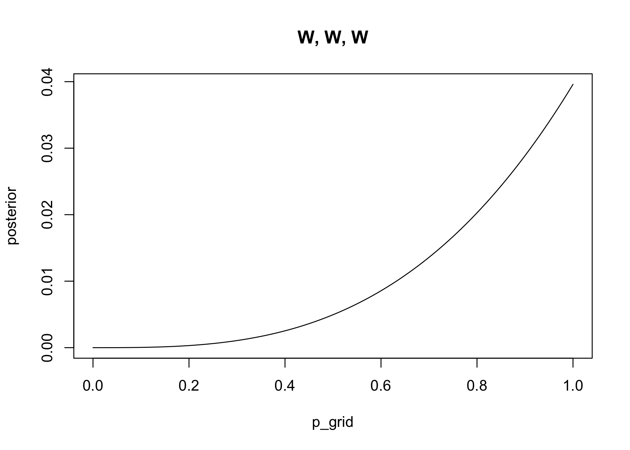
2M1: Recall the globe tossing model from the chapter. Compute and plot the grid approximate posterior distribution for each of the following sets of observations. In each case, assume a uniform prior for p.
p_grid <- seq( from=0 , to=1 , length.out=100 ) # grid from 0 to 1 with length 100
prior <- rep(1,100) # uniform prior

# likelihood of 3 water in 3 tosses
likelihood <- dbinom( 3 , size=3 , prob=p_grid )

posterior <- likelihood * prior
posterior <- posterior / sum(posterior) # standardize

plot( posterior ~ p_grid , type="l", main = "W, W, W")
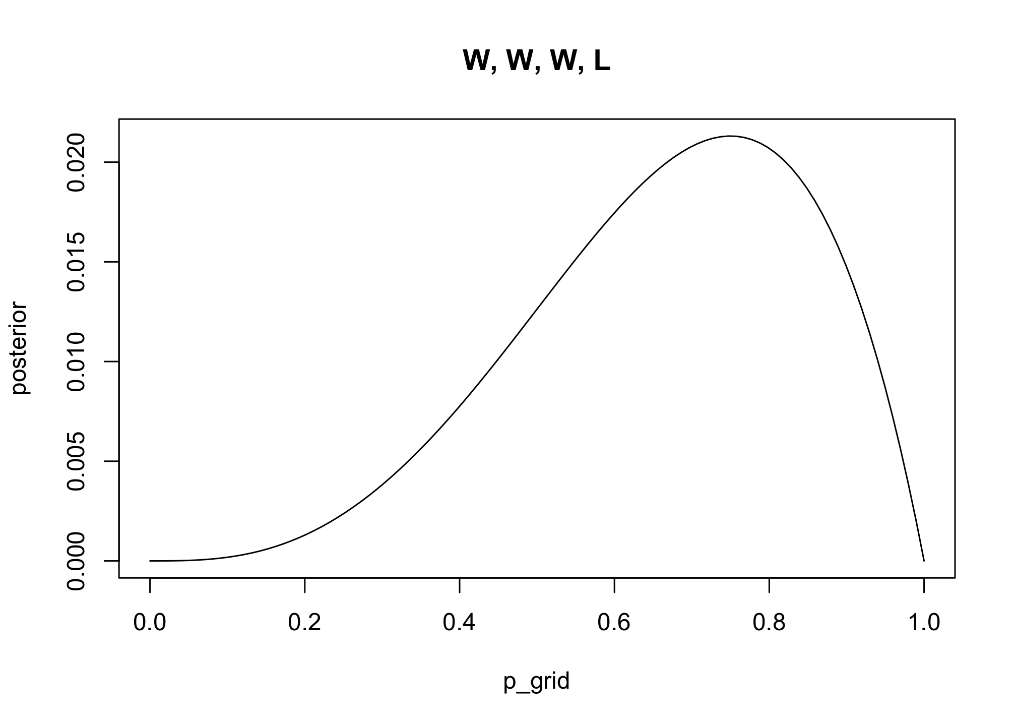
# likelihood of 3 water in 4 tosses
likelihood <- dbinom( 3 , size=4 , prob=p_grid )

posterior <- likelihood * prior
posterior <- posterior / sum(posterior) # standardize

plot( posterior ~ p_grid , type="l" , main = "W, W, W, L")
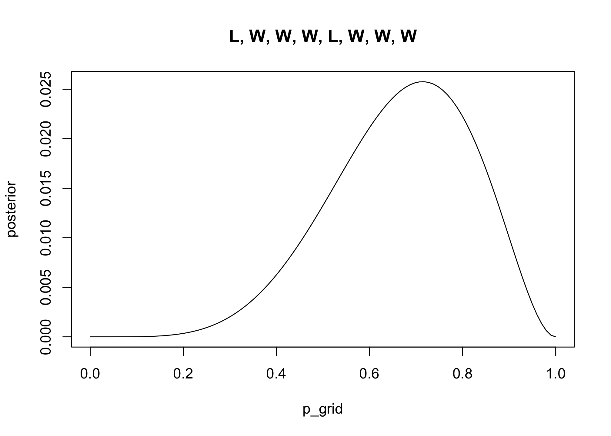
# likelihood of 5 water in 7 tosses
likelihood <- dbinom( 5 , size=7 , prob=p_grid )

posterior <- likelihood * prior
posterior <- posterior / sum(posterior) # standardize

plot( posterior ~ p_grid , type="l" , main = "L, W, W, W, L, W, W, W")
Chapter 3
Assume we have the following model:
p_grid <- seq(from = 0, to = 1, length.out = 1000)
prior <- rep(1, 1000)
likelihood <- dbinom(6, size = 9, prob = p_grid)
posterior <- likelihood * prior
posterior <- posterior / sum(posterior)

set.seed(100) # very important when using randomized functions (e.g., sample)
samples <- sample(p_grid, prob = posterior, size = 1e4, replace = TRUE)
Demo Problems
Let’s follow work in section 3.2 to understand how to summarize information from the posterior.
3E1: How much posterior probability lies below p = 0.2?
mean(samples < 0.2)
## [1] 4e-04
3E2: How much posterior probability lies above p = 0.8?
mean(samples > 0.8)
## [1] 0.1116
3E3: How much posterior probability lies between p = 0.2 and p = 0.8?
sum( samples > 0.2 & samples < 0.8 ) / 1e4
## [1] 0.888
3E4: 20% of the posterior probability lies below which value of p?
quantile(samples, probs = 0.2)
##       20%
## 0.5185185
3E5: 20% of the posterior probability lies above which value of p?
quantile(samples, probs = 0.8)
##       80%
## 0.7557558
3E6: Which values of p contain the narrowest interval equal to 66% of the posterior probability?
HPDI(samples, prob = 0.66)
##     |0.66     0.66|
## 0.5085085 0.7737738
3E7: Which values of p contain 66% of the posterior probability, assuming equal posterior probability both below and above the interval?
PI(samples, prob = 0.66)
##       17%       83%
## 0.5025025 0.7697698
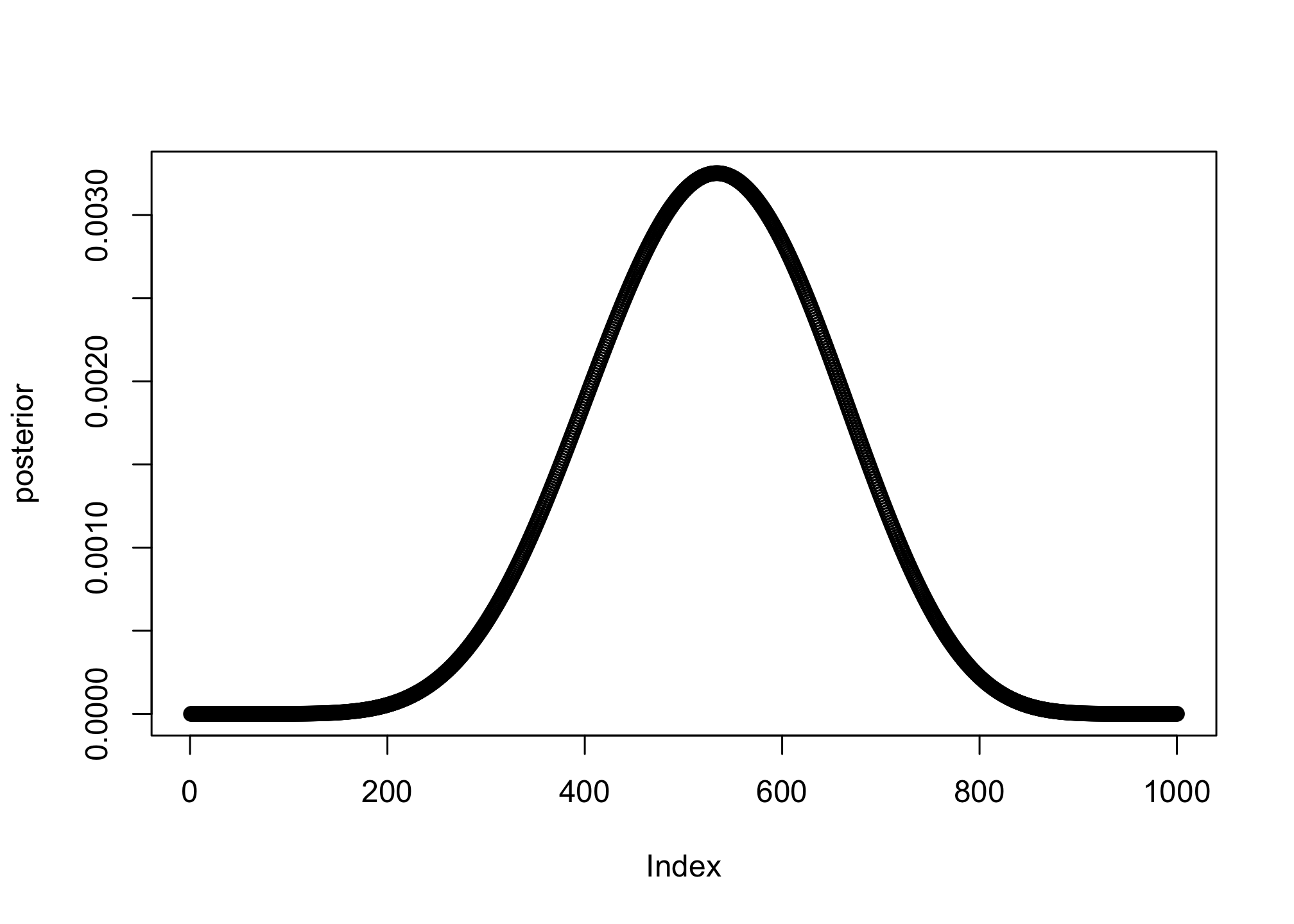
3M1: Suppose the globe tossing data had turned out to be 8 water in 15 tosses. Constructe the posterior distribution, using grid approximation. Use the same flat prior as before.
p_grid <- seq(from = 0, to = 1, length.out = 1000)
prior <- rep(1, 1000)
likelihood <- dbinom(8, size = 15, prob = p_grid)
posterior <- likelihood * prior
posterior <- posterior / sum(posterior)

plot(posterior)
3M2. Draw 10,000 samples from the grid approximation from above. Then use the sample to calculate the 90% HPDI for p.
samples <- sample(p_grid, prob = posterior, size = 1e4, replace = TRUE)

HPDI(samples, prob = 0.9)
##      |0.9      0.9|
## 0.3293293 0.7167167
3M3. Construct a posterior predictive check for this model and data. The means simulate the distribution of samples, averaging over the posterior uncertainty in p. What is the probability of observing 8 water in 15 tosses?
w <- rbinom(1e4, size = 15, prob = samples)
mean(w == 8)
## [1] 0.1444
3M4: Using the posterior distribution constructed from the new (8/15) data, now calculate the probability of observing 6 water in 9 tosses.
w <- rbinom(1e4, size = 9, prob = samples)
mean(w == 6)
## [1] 0.1751
Appendix: tidyverse conversion
Statistical Rethinking uses base R functions. More recently, Soloman Kurz has created a translation of the book’s functions into tidyverse (and later brms) code. This is not necessary but could be extremely helpful to classmates who are familiar with tidyverse already.
First, we’ll need to call tidyverse. If you do not have tidyverse, you’ll need to install it.
library(tidyverse)
For example, we can translate 2.3 code using pipes (%>%)
d <- tibble(p_grid = seq(from = 0, to = 1, length.out = 20),      # define grid
           prior  = 1) %>%                                       # define prior
    mutate(likelihood = dbinom(6, size = 9, prob = p_grid)) %>%  # compute likelihood at each value in grid
    mutate(unstd_posterior = likelihood * prior) %>%             # compute product of likelihood and prior
    mutate(posterior = unstd_posterior / sum(unstd_posterior))

d
## # A tibble: 20 × 5
##    p_grid prior likelihood unstd_posterior   posterior
##     <dbl> <dbl>      <dbl>           <dbl>       <dbl>
##  1 0          1 0               0          0
##  2 0.0526     1 0.00000152      0.00000152 0.000000799
##  3 0.105      1 0.0000819       0.0000819  0.0000431
##  4 0.158      1 0.000777        0.000777   0.000409
##  5 0.211      1 0.00360         0.00360    0.00189
##  6 0.263      1 0.0112          0.0112     0.00587
##  7 0.316      1 0.0267          0.0267     0.0140
##  8 0.368      1 0.0529          0.0529     0.0279
##  9 0.421      1 0.0908          0.0908     0.0478
## 10 0.474      1 0.138           0.138      0.0728
## 11 0.526      1 0.190           0.190      0.0999
## 12 0.579      1 0.236           0.236      0.124
## 13 0.632      1 0.267           0.267      0.140
## 14 0.684      1 0.271           0.271      0.143
## 15 0.737      1 0.245           0.245      0.129
## 16 0.789      1 0.190           0.190      0.0999
## 17 0.842      1 0.118           0.118      0.0621
## 18 0.895      1 0.0503          0.0503     0.0265
## 19 0.947      1 0.00885         0.00885    0.00466
## 20 1          1 0               0          0
With this calculated, we can then use ggplot2, the staple ggplot2 data visualization package, to plot our posterior.
d %>%
  ggplot(aes(x = p_grid, y = posterior)) +
  geom_point() +
  geom_line() +
  labs(subtitle = "20 points",
       x = "probability of water",
       y = "posterior probability") +
  theme(panel.grid = element_blank())
For this class, we’ll occasionally refer to Soloman’s guide.
Demo Problem
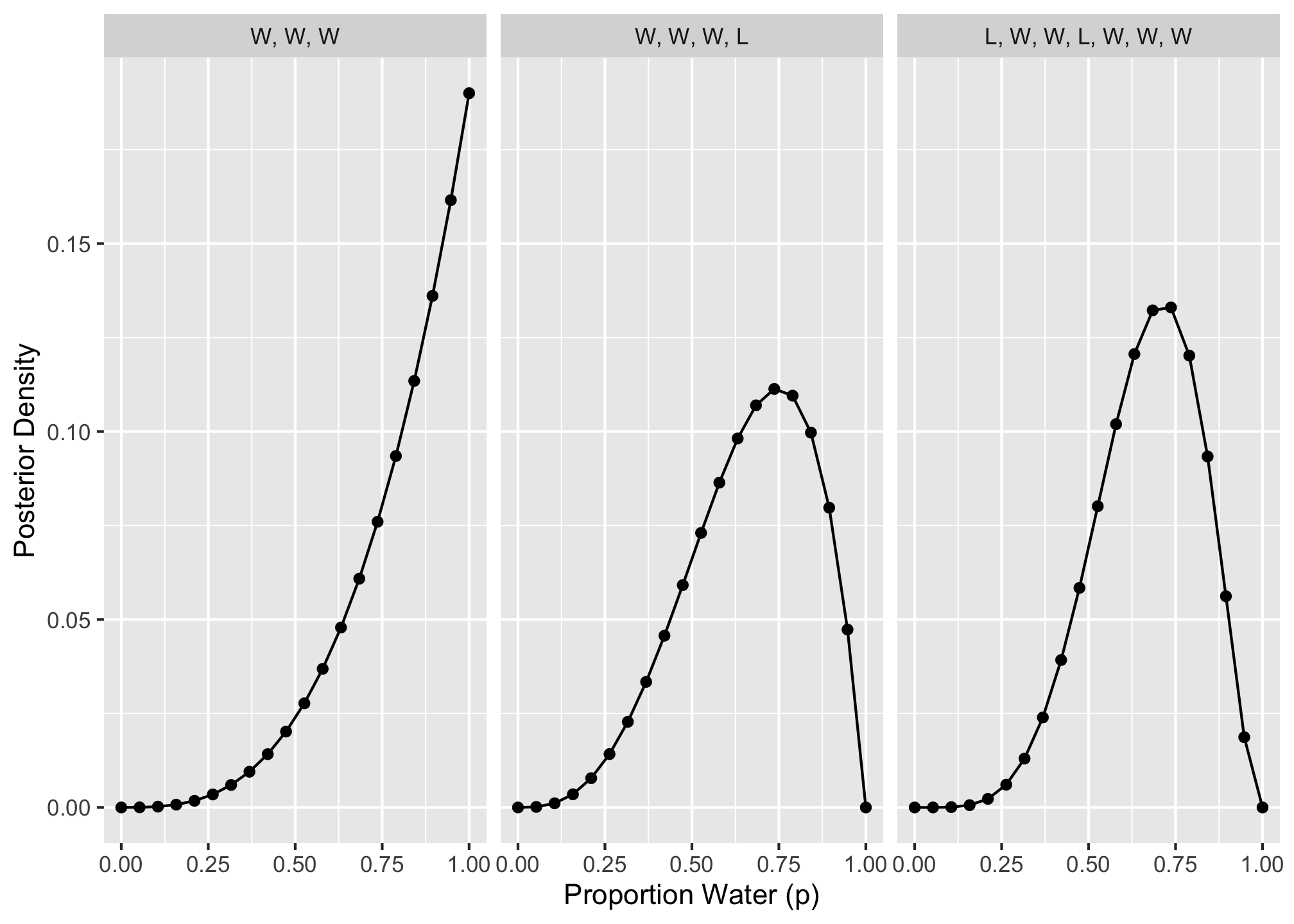
2M1: Recall the globe tossing model from the chapter. Compute and plot the grid approximate posterior distribution for each of the following sets of observations. In each case, assume a uniform prior for p.
## be sure to have tidyverse installed, i.e., install.packages('tidyverse')
library(tidyverse)

dist <- tibble(p_grid = seq(from = 0, to = 1, length.out = 20),
               prior = rep(1, times = 20)) %>%
  mutate(likelihood_1 = dbinom(3, size = 3, prob = p_grid),
         likelihood_2 = dbinom(3, size = 4, prob = p_grid),
         likelihood_3 = dbinom(5, size = 7, prob = p_grid),
         across(starts_with("likelihood"), ~ .x * prior),
         across(starts_with("likelihood"), ~ .x / sum(.x))) %>%
  pivot_longer(cols = starts_with("likelihood"), names_to = "pattern",
               values_to = "posterior") %>%
  separate(pattern, c(NA, "pattern"), sep = "_", convert = TRUE) %>%
  mutate(obs = case_when(pattern == 1L ~ "W, W, W",
                         pattern == 2L ~ "W, W, W, L",
                         pattern == 3L ~ "L, W, W, L, W, W, W"))

ggplot(dist, aes(x = p_grid, y = posterior)) +
  facet_wrap(vars(fct_inorder(obs)), nrow = 1) +
  geom_line() +
  geom_point() +
  labs(x = "Proportion Water (p)", y = "Posterior Density")
# W, W, W, L, W, W, W

# challenge: functionalize this to generalize this for any read in toss string

d2m1 <- tibble(p_grid = seq(from = 0, to = 1, length.out = 20),
               prior = rep(1, times = 20)) %>%
  mutate(
         likelihood_1 = dbinom(1, size = 1, prob = p_grid),
         likelihood_2 = dbinom(2, size = 2, prob = p_grid),
         likelihood_3 = dbinom(3, size = 3, prob = p_grid),
         likelihood_4 = dbinom(3, size = 4, prob = p_grid),
         likelihood_5 = dbinom(4, size = 5, prob = p_grid),
         likelihood_6 = dbinom(5, size = 6, prob = p_grid),
         likelihood_7 = dbinom(6, size = 7, prob = p_grid),
         across(starts_with("likelihood"), ~ .x * prior),
         across(starts_with("likelihood"), ~ .x / sum(.x))) %>%
  pivot_longer(cols = starts_with("likelihood"), names_to = "pattern",
               values_to = "posterior") %>%
  separate(pattern, c(NA, "pattern"), sep = "_", convert = TRUE) %>%
  mutate(obs = case_when(pattern == 1L ~ "W",
                         pattern == 2L ~ "W, W",
                         pattern == 3L ~ "W, W, W,",
                         pattern == 4L ~ "W, W, W, L",
                         pattern == 5L ~ "W, W, W, L, W",
                         pattern == 6L ~ "W, W, W, L, W, W",
                         pattern == 7L ~ "W, W, W, L, W, W, W"))

d2m1
## # A tibble: 140 × 5
##    p_grid prior pattern posterior obs
##     <dbl> <dbl>   <int>     <dbl> <chr>
##  1 0          1       1 0         W
##  2 0          1       2 0         W, W
##  3 0          1       3 0         W, W, W,
##  4 0          1       4 0         W, W, W, L
##  5 0          1       5 0         W, W, W, L, W
##  6 0          1       6 0         W, W, W, L, W, W
##  7 0          1       7 0         W, W, W, L, W, W, W
##  8 0.0526     1       1 0.00526   W
##  9 0.0526     1       2 0.000405  W, W
## 10 0.0526     1       3 0.0000277 W, W, W,
## # … with 130 more rows
# be sure to install gganimate, i.e., run install.packages('gganimate')
library(gganimate)

anim <- ggplot(d2m1, aes(x = p_grid, y = posterior, group = obs)) +
  geom_point() +
  geom_line() +
  theme(legend.position = "none") +
  transition_states(obs,
                    transition_length = 2,
                    state_length = 1) +
  labs(x = "Proportion Water (p)", y = "Posterior Probability") +
  ggtitle('Toss Result: {closest_state}') +
  enter_fade() +
  exit_fade()

animate(anim, height = 500, width = 600)
#anim_save("../../static/img/example/World-tossing-bayesian-chapter2.gif")

Package versions
sessionInfo()
## R version 4.1.1 (2021-08-10)
## Platform: aarch64-apple-darwin20 (64-bit)
## Running under: macOS Monterey 12.1
##
## Matrix products: default
## BLAS:   /Library/Frameworks/R.framework/Versions/4.1-arm64/Resources/lib/libRblas.0.dylib
## LAPACK: /Library/Frameworks/R.framework/Versions/4.1-arm64/Resources/lib/libRlapack.dylib
##
## locale:
## [1] en_US.UTF-8/en_US.UTF-8/en_US.UTF-8/C/en_US.UTF-8/en_US.UTF-8
##
## attached base packages:
## [1] parallel  stats     graphics  grDevices datasets  utils     methods
## [8] base
##
## other attached packages:
##  [1] gganimate_1.0.7      forcats_0.5.1        stringr_1.4.0
##  [4] dplyr_1.0.7          purrr_0.3.4          readr_2.0.2
##  [7] tidyr_1.1.4          tibble_3.1.6         tidyverse_1.3.1
## [10] rethinking_2.21      cmdstanr_0.4.0.9001  rstan_2.21.3
## [13] ggplot2_3.3.5        StanHeaders_2.21.0-7
##
## loaded via a namespace (and not attached):
##   [1] colorspace_2.0-2     class_7.3-19         ellipsis_0.3.2
##   [4] base64enc_0.1-3      fs_1.5.0             xaringanExtra_0.5.5
##   [7] rstudioapi_0.13      proxy_0.4-26         farver_2.1.0
##  [10] fansi_0.5.0          mvtnorm_1.1-3        lubridate_1.8.0
##  [13] xml2_1.3.2           codetools_0.2-18     knitr_1.36
##  [16] jsonlite_1.7.2       bsplus_0.1.3         broom_0.7.9
##  [19] dbplyr_2.1.1         compiler_4.1.1       httr_1.4.2
##  [22] backports_1.4.1      assertthat_0.2.1     fastmap_1.1.0
##  [25] cli_3.1.0            tweenr_1.0.2         htmltools_0.5.2
##  [28] prettyunits_1.1.1    tools_4.1.1          coda_0.19-4
##  [31] gtable_0.3.0         glue_1.6.0           posterior_1.1.0
##  [34] Rcpp_1.0.7           cellranger_1.1.0     jquerylib_0.1.4
##  [37] vctrs_0.3.8          blogdown_1.5         transformr_0.1.3
##  [40] tensorA_0.36.2       xfun_0.28            ps_1.6.0
##  [43] rvest_1.0.2          mime_0.12            lpSolve_5.6.15
##  [46] lifecycle_1.0.1      renv_0.14.0          MASS_7.3-54
##  [49] scales_1.1.1         hms_1.1.1            inline_0.3.19
##  [52] yaml_2.2.1           gridExtra_2.3        downloadthis_0.2.1
##  [55] loo_2.4.1            sass_0.4.0           stringi_1.7.6
##  [58] highr_0.9            e1071_1.7-9          checkmate_2.0.0
##  [61] pkgbuild_1.3.1       shape_1.4.6          rlang_0.4.12
##  [64] pkgconfig_2.0.3      matrixStats_0.61.0   distributional_0.2.2
##  [67] evaluate_0.14        lattice_0.20-44      sf_1.0-5
##  [70] labeling_0.4.2       processx_3.5.2       tidyselect_1.1.1
##  [73] plyr_1.8.6           magrittr_2.0.1       bookdown_0.24
##  [76] R6_2.5.1             magick_2.7.3         generics_0.1.1
##  [79] DBI_1.1.1            pillar_1.6.4         haven_2.4.3
##  [82] withr_2.4.3          units_0.7-2          abind_1.4-5
##  [85] modelr_0.1.8         crayon_1.4.2         KernSmooth_2.23-20
##  [88] uuid_1.0-3           utf8_1.2.2           tzdb_0.1.2
##  [91] rmarkdown_2.11       progress_1.2.2       grid_4.1.1
##  [94] readxl_1.3.1         callr_3.7.0          reprex_2.0.1
##  [97] digest_0.6.29        classInt_0.4-3       RcppParallel_5.1.4
## [100] stats4_4.1.1         munsell_0.5.0        bslib_0.3.1