Class 2
Introduction
For this class, we’ll review code examples found in Chapter 2.
This assumes that you have already installed the rethinking package.
If you need help, be sure to remember the references in the Resources:
Bayesian Updating: Grid Approximation
Let’s assume we have the table in 2.1
## R code 2.1
ways <- c( 0 , 3 , 8 , 9 , 0 )
ways/sum(ways)
## [1] 0.00 0.15 0.40 0.45 0.00Let’s compute the likelihood of six W’s in nine tosses (assuming a 50% probability):
## R code 2.2
dbinom( 6 , size=9 , prob=0.5 )
## [1] 0.1640625We can see it’s 16.4%.
Be sure to examine the dbinom function by typing in ?dbinom and exploring the documentation. We’ll use this function a lot in this class.
Next, let’s define a grid. This is required when we are using Grid Approximation for our Bayesian calculations (i.e., to estimate the posterior).
## R code 2.3
# define grid
p_grid <- seq( from=0 , to=1 , length.out=20 )

p_grid
## [1] 0.00000000 0.05263158 0.10526316 0.15789474 0.21052632 0.26315789
## [7] 0.31578947 0.36842105 0.42105263 0.47368421 0.52631579 0.57894737
## [13] 0.63157895 0.68421053 0.73684211 0.78947368 0.84210526 0.89473684
## [19] 0.94736842 1.00000000Notice that this function creates a vector with length 20 and that ranges from 0 to 1. Note as well that each vector element is evenly spaced in increments of (to - from)/(length.out - 1).
Think about the trade-off between having a smaller or larger length.out.
Next, let’s define our prior. We’ll assume a “flat” prior.
# define prior
prior <- rep( 1 , 20 )

prior
## [1] 1 1 1 1 1 1 1 1 1 1 1 1 1 1 1 1 1 1 1 1# compute likelihood at each value in grid
likelihood <- dbinom( 6 , size=9 , prob=p_grid )
likelihood## [1] 0.000000e+00 1.518149e-06 8.185093e-05 7.772923e-04 3.598575e-03
## [6] 1.116095e-02 2.668299e-02 5.292110e-02 9.082698e-02 1.383413e-01
## [11] 1.897686e-01 2.361147e-01 2.666113e-01 2.714006e-01 2.450051e-01
## [16] 1.897686e-01 1.179181e-01 5.026670e-02 8.853845e-03 0.000000e+00# compute product of likelihood and prior
unstd.posterior <- likelihood * prior
unstd.posterior## [1] 0.000000e+00 1.518149e-06 8.185093e-05 7.772923e-04 3.598575e-03
## [6] 1.116095e-02 2.668299e-02 5.292110e-02 9.082698e-02 1.383413e-01
## [11] 1.897686e-01 2.361147e-01 2.666113e-01 2.714006e-01 2.450051e-01
## [16] 1.897686e-01 1.179181e-01 5.026670e-02 8.853845e-03 0.000000e+00# standardize the posterior, so it sums to 1
posterior <- unstd.posterior / sum(unstd.posterior)
posterior## [1] 0.000000e+00 7.989837e-07 4.307717e-05 4.090797e-04 1.893887e-03
## [6] 5.873873e-03 1.404294e-02 2.785174e-02 4.780115e-02 7.280739e-02
## [11] 9.987296e-02 1.242643e-01 1.403143e-01 1.428349e-01 1.289433e-01
## [16] 9.987296e-02 6.205890e-02 2.645477e-02 4.659673e-03 0.000000e+00## R code 2.4
plot( p_grid , posterior , type="b" ,
xlab="probability of water" , ylab="posterior probability" )
mtext( "20 points" )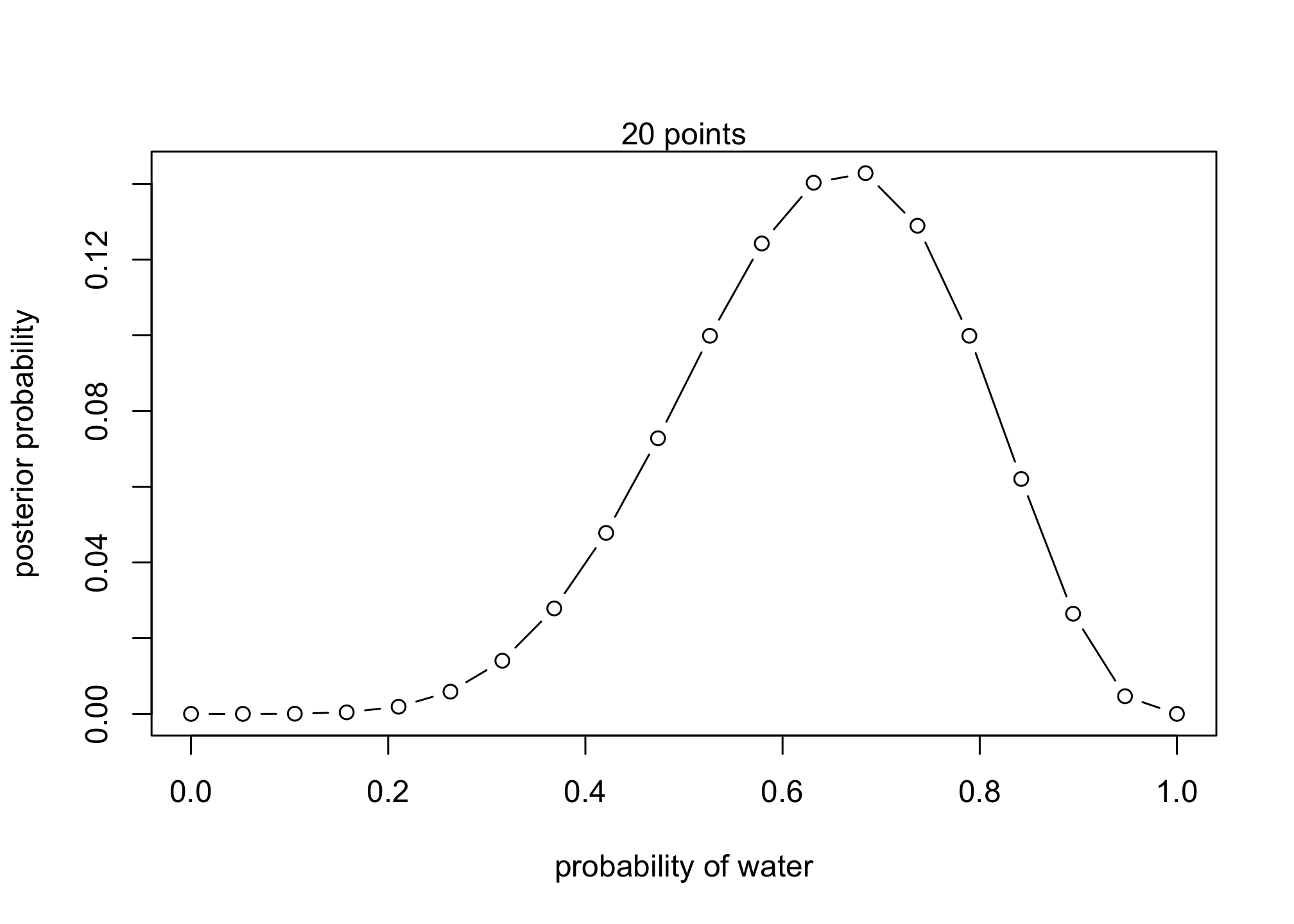 What happens if we alter the priors? What will be the new posteriors?
## R code 2.5
prior <- ifelse( p_grid < 0.5 , 0 , 1 )
prior <- exp( -5*abs( p_grid - 0.5 ) )
Bayesian Updating: Quadratic Approximation
## R code 2.6
library(rethinking)
globe.qa <- quap(
    alist(
        W ~ dbinom( W+L ,p) ,  # binomial likelihood
        p ~ dunif(0,1)     # uniform prior
    ) ,
    data=list(W=6,L=3) )

# display summary of quadratic approximation
precis( globe.qa )
## mean sd 5.5% 94.5%
## p 0.6666662 0.1571339 0.4155358 0.9177965## R code 2.7
# analytical calculation
W <- 6
L <- 3
curve( dbeta( x , W+1 , L+1 ) , from=0 , to=1 )
# quadratic approximation
curve( dnorm( x , 0.67 , 0.16 ) , lty=2 , add=TRUE )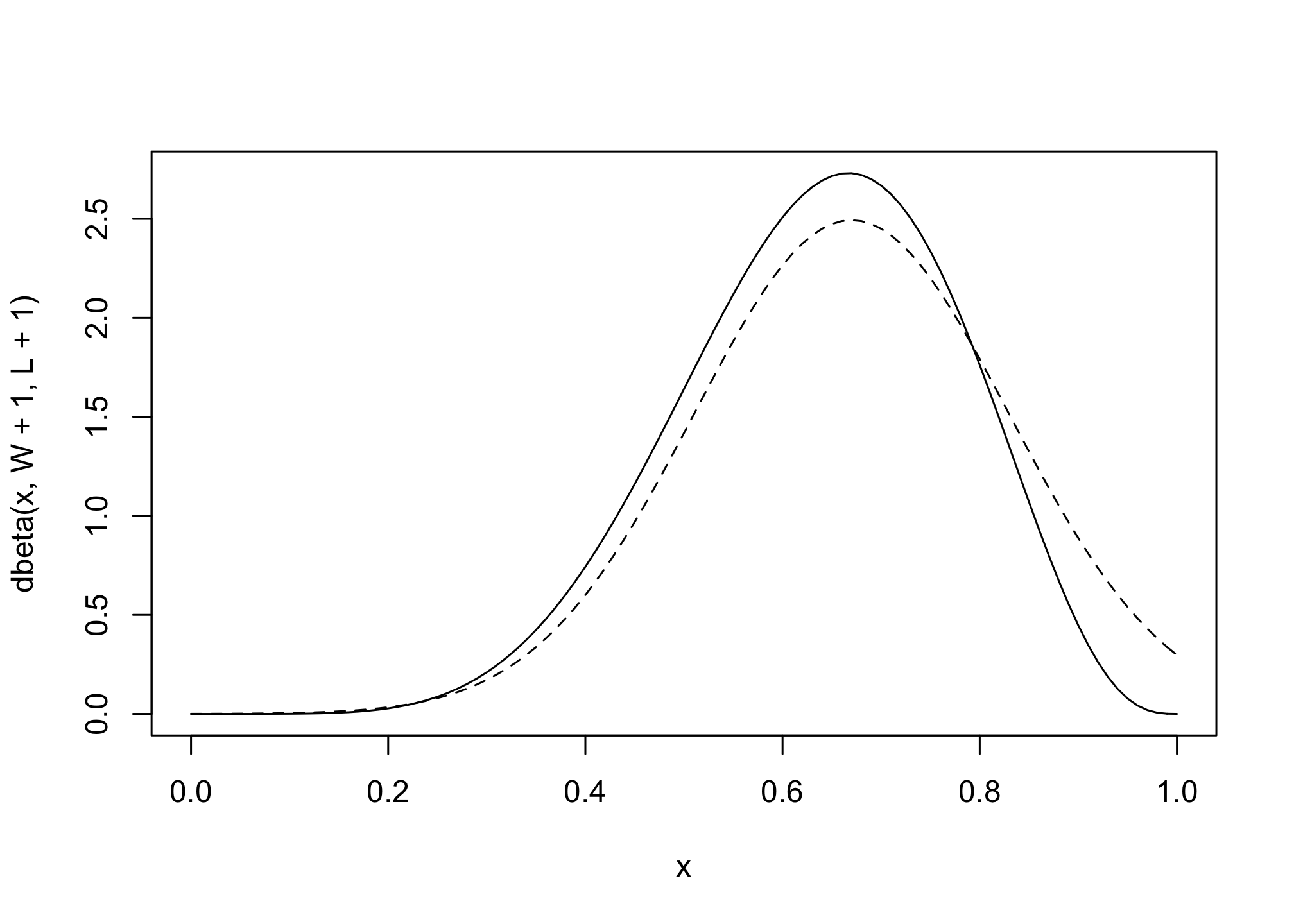
## R code 2.8
n_samples <- 1000
p <- rep( NA , n_samples )
p[1] <- 0.5
W <- 6
L <- 3
for ( i in 2:n_samples ) {
    p_new <- rnorm( 1 , p[i-1] , 0.1 )
    if ( p_new < 0 ) p_new <- abs( p_new )
    if ( p_new > 1 ) p_new <- 2 - p_new
    q0 <- dbinom( W , W+L , p[i-1] )
    q1 <- dbinom( W , W+L , p_new )
    p[i] <- ifelse( runif(1) < q1/q0 , p_new , p[i-1] )
}

## R code 2.9
dens( p , xlim=c(0,1) )
curve( dbeta( x , W+1 , L+1 ) , lty=2 , add=TRUE )
tidyverse conversion
Statistical Rethinking uses base R functions. More recently, Soloman Kurz has created a translation of the book’s functions into tidyverse (and later brms) code. This is not necessary but could be extremely helpful to classmates who are familiar with tidyverse already.
First, we’ll need to call tidyverse. If you do not have tidyverse, you’ll need to install it.
library(tidyverse)For example, we can translate 2.3 code using pipes (%>%)
d <- tibble(p_grid = seq(from = 0, to = 1, length.out = 20),      # define grid
           prior  = 1) %>%                                       # define prior
    mutate(likelihood = dbinom(6, size = 9, prob = p_grid)) %>%  # compute likelihood at each value in grid
    mutate(unstd_posterior = likelihood * prior) %>%             # compute product of likelihood and prior
    mutate(posterior = unstd_posterior / sum(unstd_posterior))

d
## # A tibble: 20 × 5
## p_grid prior likelihood unstd_posterior posterior
## <dbl> <dbl> <dbl> <dbl> <dbl>
## 1 0 1 0 0 0
## 2 0.0526 1 0.00000152 0.00000152 0.000000799
## 3 0.105 1 0.0000819 0.0000819 0.0000431
## 4 0.158 1 0.000777 0.000777 0.000409
## 5 0.211 1 0.00360 0.00360 0.00189
## 6 0.263 1 0.0112 0.0112 0.00587
## 7 0.316 1 0.0267 0.0267 0.0140
## 8 0.368 1 0.0529 0.0529 0.0279
## 9 0.421 1 0.0908 0.0908 0.0478
## 10 0.474 1 0.138 0.138 0.0728
## 11 0.526 1 0.190 0.190 0.0999
## 12 0.579 1 0.236 0.236 0.124
## 13 0.632 1 0.267 0.267 0.140
## 14 0.684 1 0.271 0.271 0.143
## 15 0.737 1 0.245 0.245 0.129
## 16 0.789 1 0.190 0.190 0.0999
## 17 0.842 1 0.118 0.118 0.0621
## 18 0.895 1 0.0503 0.0503 0.0265
## 19 0.947 1 0.00885 0.00885 0.00466
## 20 1 1 0 0 0With this calculated, we can then use ggplot2, the staple ggplot2 data visualization package, to plot our posterior.
d %>%
  ggplot(aes(x = p_grid, y = posterior)) +
  geom_point() +
  geom_line() +
  labs(subtitle = "20 points",
       x = "probability of water",
       y = "posterior probability") +
  theme(panel.grid = element_blank())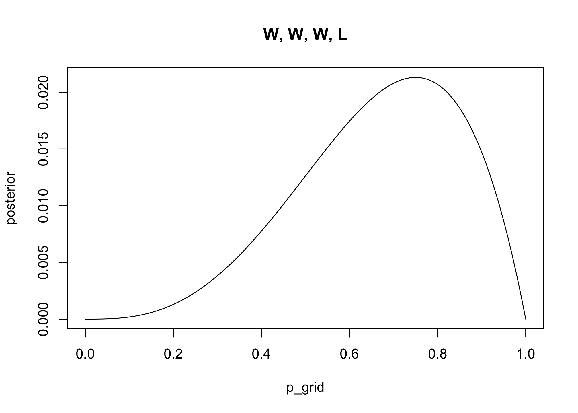
For this class, we’ll occasionally refer to Soloman’s guide.
Practice Problems
2M1: Recall the globe tossing model from the chapter. Compute and plot the grid approximate posterior distribution for each of the following sets of observations. In each case, assume a uniform prior for p.
library(tidyverse)

dist <- tibble(p_grid = seq(from = 0, to = 1, length.out = 20),
               prior = rep(1, times = 20)) %>%
  mutate(likelihood_1 = dbinom(3, size = 3, prob = p_grid),
         likelihood_2 = dbinom(3, size = 4, prob = p_grid),
         likelihood_3 = dbinom(5, size = 7, prob = p_grid),
         across(starts_with("likelihood"), ~ .x * prior),
         across(starts_with("likelihood"), ~ .x / sum(.x))) %>%
  pivot_longer(cols = starts_with("likelihood"), names_to = "pattern",
               values_to = "posterior") %>%
  separate(pattern, c(NA, "pattern"), sep = "_", convert = TRUE) %>%
  mutate(obs = case_when(pattern == 1L ~ "W, W, W",
                         pattern == 2L ~ "W, W, W, L",
                         pattern == 3L ~ "L, W, W, L, W, W, W"))

ggplot(dist, aes(x = p_grid, y = posterior)) +
  facet_wrap(vars(fct_inorder(obs)), nrow = 1) +
  geom_line() +
  geom_point() +
  labs(x = "Proportion Water (p)", y = "Posterior Density")
# W, W, W, L, W, W, W

# challenge: functionalize this to generalize this for any read in toss string

d2m1 <- tibble(p_grid = seq(from = 0, to = 1, length.out = 20),
               prior = rep(1, times = 20)) %>%
  mutate(
         likelihood_1 = dbinom(1, size = 1, prob = p_grid),
         likelihood_2 = dbinom(2, size = 2, prob = p_grid),
         likelihood_3 = dbinom(3, size = 3, prob = p_grid),
         likelihood_4 = dbinom(3, size = 4, prob = p_grid),
         likelihood_5 = dbinom(4, size = 5, prob = p_grid),
         likelihood_6 = dbinom(5, size = 6, prob = p_grid),
         likelihood_7 = dbinom(6, size = 7, prob = p_grid),
         across(starts_with("likelihood"), ~ .x * prior),
         across(starts_with("likelihood"), ~ .x / sum(.x))) %>%
  pivot_longer(cols = starts_with("likelihood"), names_to = "pattern",
               values_to = "posterior") %>%
  separate(pattern, c(NA, "pattern"), sep = "_", convert = TRUE) %>%
  mutate(obs = case_when(pattern == 1L ~ "W",
                         pattern == 2L ~ "W, W",
                         pattern == 3L ~ "W, W, W,",
                         pattern == 4L ~ "W, W, W, L",
                         pattern == 5L ~ "W, W, W, L, W",
                         pattern == 6L ~ "W, W, W, L, W, W",
                         pattern == 7L ~ "W, W, W, L, W, W, W"))

d2m1
## # A tibble: 140 × 5
## p_grid prior pattern posterior obs
## <dbl> <dbl> <int> <dbl> <chr>
## 1 0 1 1 0 W
## 2 0 1 2 0 W, W
## 3 0 1 3 0 W, W, W,
## 4 0 1 4 0 W, W, W, L
## 5 0 1 5 0 W, W, W, L, W
## 6 0 1 6 0 W, W, W, L, W, W
## 7 0 1 7 0 W, W, W, L, W, W, W
## 8 0.0526 1 1 0.00526 W
## 9 0.0526 1 2 0.000405 W, W
## 10 0.0526 1 3 0.0000277 W, W, W,
## # … with 130 more rowslibrary(gganimate)
anim <- ggplot(d2m1, aes(x = p_grid, y = posterior, group = obs)) +
geom_point() +
geom_line() +
theme(legend.position = "none") +
transition_states(obs,
transition_length = 2,
state_length = 1) +
labs(x = "Proportion Water (p)", y = "Posterior Probability") +
ggtitle('Toss Result: {closest_state}') +
enter_fade() +
exit_fade()
animate(anim, height = 500, width = 600)
#anim_save("World-tossing-bayesian-chapter2.gif")Package versions
sessionInfo()## R version 4.1.1 (2021-08-10)
## Platform: aarch64-apple-darwin20 (64-bit)
## Running under: macOS Monterey 12.1
##
## Matrix products: default
## BLAS: /Library/Frameworks/R.framework/Versions/4.1-arm64/Resources/lib/libRblas.0.dylib
## LAPACK: /Library/Frameworks/R.framework/Versions/4.1-arm64/Resources/lib/libRlapack.dylib
##
## locale:
## [1] en_US.UTF-8/en_US.UTF-8/en_US.UTF-8/C/en_US.UTF-8/en_US.UTF-8
##
## attached base packages:
## [1] parallel stats graphics grDevices datasets utils methods
## [8] base
##
## other attached packages:
## [1] gganimate_1.0.7 forcats_0.5.1 stringr_1.4.0
## [4] dplyr_1.0.7 purrr_0.3.4 readr_2.0.2
## [7] tidyr_1.1.4 tibble_3.1.6 tidyverse_1.3.1
## [10] rethinking_2.21 cmdstanr_0.4.0.9001 rstan_2.21.3
## [13] ggplot2_3.3.5 StanHeaders_2.21.0-7
##
## loaded via a namespace (and not attached):
## [1] colorspace_2.0-2 class_7.3-19 ellipsis_0.3.2
## [4] base64enc_0.1-3 fs_1.5.0 xaringanExtra_0.5.5
## [7] rstudioapi_0.13 proxy_0.4-26 farver_2.1.0
## [10] fansi_0.5.0 mvtnorm_1.1-3 lubridate_1.8.0
## [13] xml2_1.3.2 codetools_0.2-18 knitr_1.36
## [16] jsonlite_1.7.2 bsplus_0.1.3 broom_0.7.9
## [19] dbplyr_2.1.1 compiler_4.1.1 httr_1.4.2
## [22] backports_1.4.1 assertthat_0.2.1 fastmap_1.1.0
## [25] cli_3.1.0 tweenr_1.0.2 htmltools_0.5.2
## [28] prettyunits_1.1.1 tools_4.1.1 coda_0.19-4
## [31] gtable_0.3.0 glue_1.6.0 posterior_1.1.0
## [34] Rcpp_1.0.7 cellranger_1.1.0 jquerylib_0.1.4
## [37] vctrs_0.3.8 blogdown_1.5 transformr_0.1.3
## [40] tensorA_0.36.2 xfun_0.28 ps_1.6.0
## [43] rvest_1.0.2 mime_0.12 lpSolve_5.6.15
## [46] lifecycle_1.0.1 renv_0.14.0 MASS_7.3-54
## [49] scales_1.1.1 hms_1.1.1 inline_0.3.19
## [52] yaml_2.2.1 gridExtra_2.3 downloadthis_0.2.1
## [55] loo_2.4.1 sass_0.4.0 stringi_1.7.6
## [58] highr_0.9 e1071_1.7-9 checkmate_2.0.0
## [61] pkgbuild_1.3.1 shape_1.4.6 rlang_0.4.12
## [64] pkgconfig_2.0.3 matrixStats_0.61.0 distributional_0.2.2
## [67] evaluate_0.14 lattice_0.20-44 sf_1.0-5
## [70] labeling_0.4.2 processx_3.5.2 tidyselect_1.1.1
## [73] plyr_1.8.6 magrittr_2.0.1 bookdown_0.24
## [76] R6_2.5.1 magick_2.7.3 generics_0.1.1
## [79] DBI_1.1.1 pillar_1.6.4 haven_2.4.3
## [82] withr_2.4.3 units_0.7-2 abind_1.4-5
## [85] modelr_0.1.8 crayon_1.4.2 KernSmooth_2.23-20
## [88] uuid_1.0-3 utf8_1.2.2 tzdb_0.1.2
## [91] rmarkdown_2.11 progress_1.2.2 grid_4.1.1
## [94] readxl_1.3.1 callr_3.7.0 reprex_2.0.1
## [97] digest_0.6.29 classInt_0.4-3 RcppParallel_5.1.4
## [100] stats4_4.1.1 munsell_0.5.0 bslib_0.3.1