Problem Set 7 Solutions
This problem set is due on April 4, 2022 at 11:59am.
Question 1
Conduct a prior predictive simulation for the Reedfrog model. By this I mean to simulate the prior distribution of tank survival probabilities \(\alpha_{j}\).
Start by using these priors:
\(\alpha_{j} \sim Normal(\bar{\alpha},\sigma)\)
\(\bar{\alpha} \sim Normal(0, 1)\)
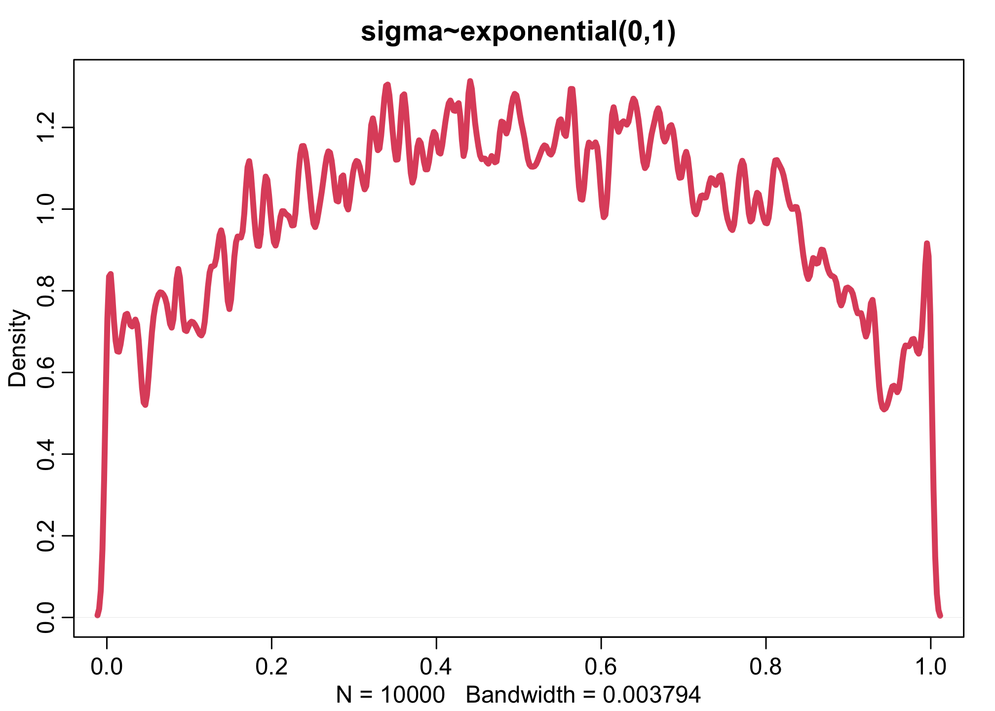
\(\sigma \sim Exponential(1)\)
Be sure to transform the \(\alpha_{j}\) values to the probability scale for plotting and summary.
How does increasing the width of the prior on σ change the prior distribution of \(\alpha_{j}\)?
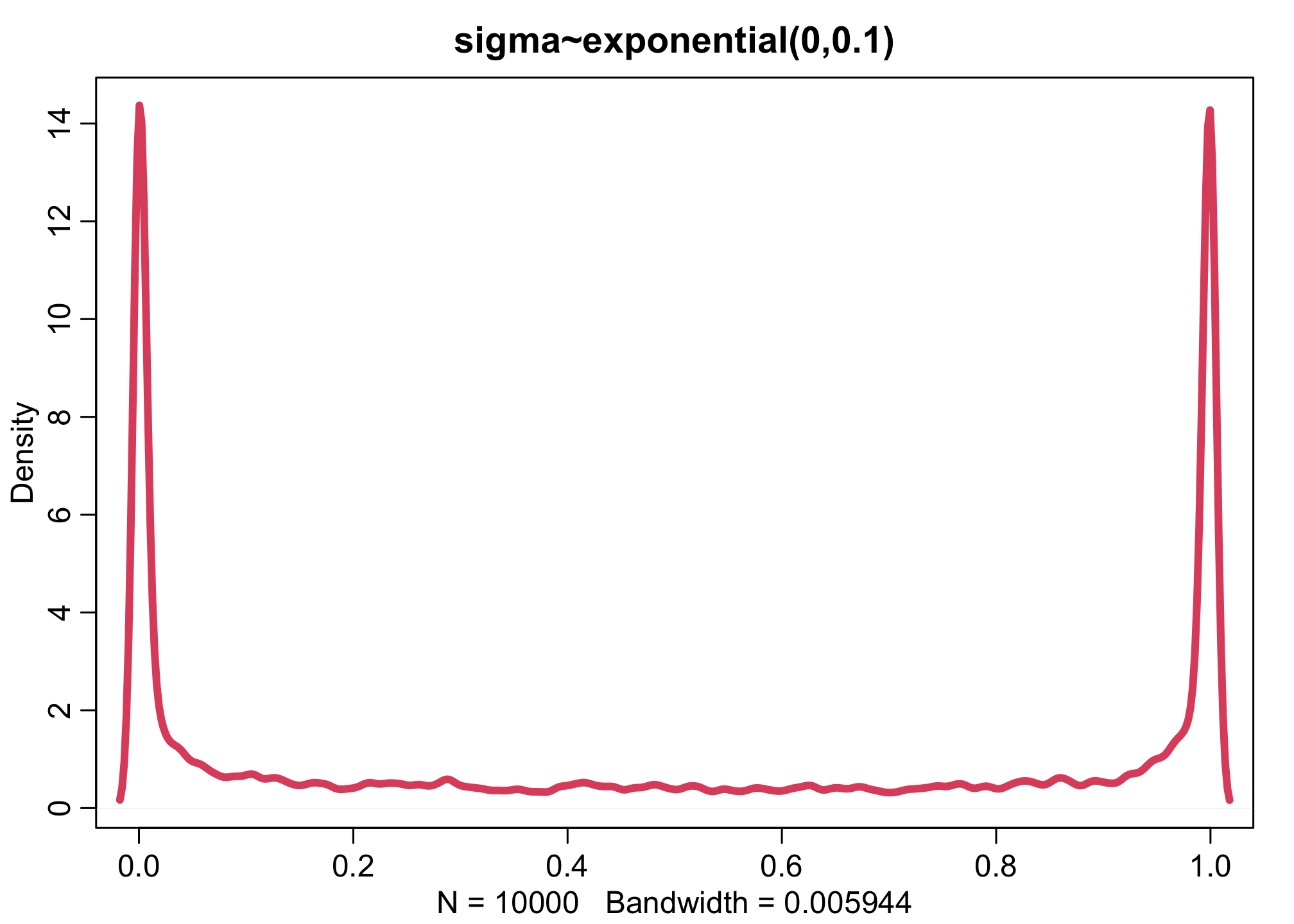
You might try Exponential(10) and Exponential(0.1) for example.
Simulating varying effect priors is in principle like simulating any other priors. The only difference is that the parameters have an implied order now, because some parameters depend upon others. So in this problem we must simulate \(\sigma\) and \(\bar{\alpha}\) first, and then we can simulate the individual tank \(\alpha_{T}\) variables
library(rethinking)
n <- 1e4
sigma <- rexp(n,1)
abar <- rnorm(n,0,1)
aT <- rnorm(n,abar,sigma)
dens(inv_logit(aT),xlim=c(0,1),adj=0.1,lwd=4,col=2, main="sigma~exponential(0,1)")
Let’s also run two more (0.1 and 10):
n <- 1e4
sigma <- rexp(n,0.1)
abar <- rnorm(n,0,1)
aT <- rnorm(n,abar,sigma)
dens(inv_logit(aT),xlim=c(0,1),adj=0.1,lwd=4,col=2, main="sigma~exponential(0,0.1)")
n <- 1e4
sigma <- rexp(n,10)
abar <- rnorm(n,0,1)
aT <- rnorm(n,abar,sigma)
dens(inv_logit(aT),xlim=c(0,1),adj=0.1,lwd=4,col=2, main="sigma~exponential(0,10)")
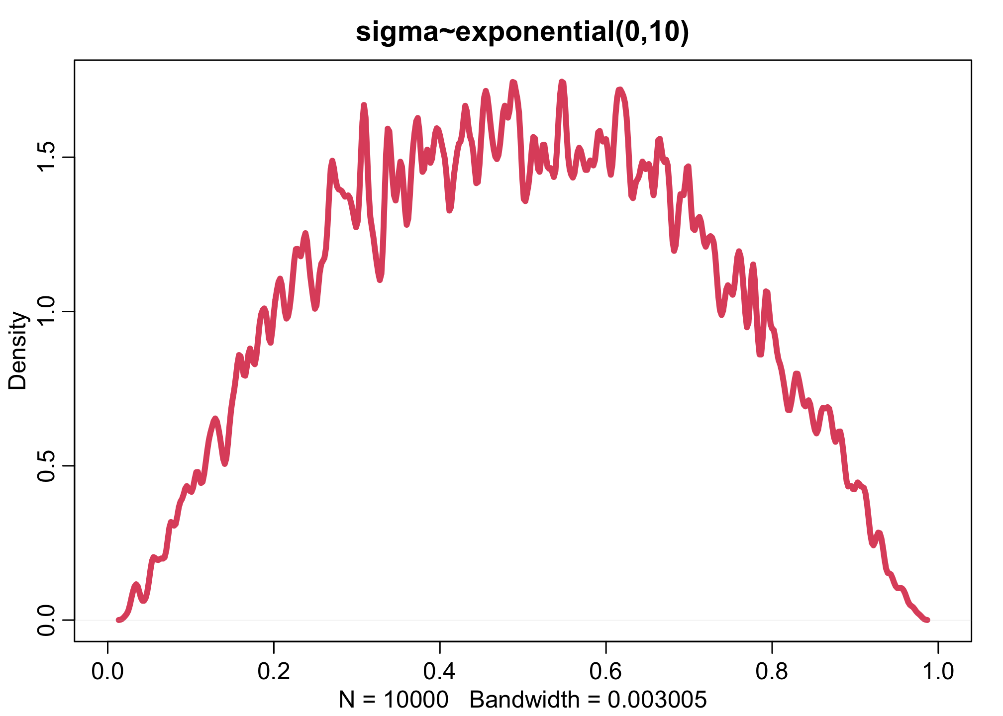
Increasing the variation across tanks, by making the \(\sigma\) distribution wider, pushes prior survival up against the floor and ceiling of the outcome space. This is the same phenomenon you saw before for ordinary logit models. The key lesson again is that flat priors on one scale are not necessarily flat on another.
Question 2
Revisit the Reedfrog survival data, data(reedfrogs). Start with the varying effects model from the book and lecture. Then modify it to estimate the causal effects of the treatment variables pred and size, including how size might modify the effect of predation. An easy approach is to estimate an effect for each combination of pred and size. Justify your model with a DAG of this experiment.
library(rethinking)
data(reedfrogs)
d <- reedfrogs

dat <- list(
S = d$surv,
D = d$density,
T = 1:nrow(d),
P = ifelse( d$pred=="no" , 1L , 2L ),
G = ifelse( d$size=="small" , 1L , 2L ) )

m2 <- ulam(
  alist(
    S ~ binomial( D , p ),
    logit(p) <- a[T] + b[P,G],
    a[T] ~ normal( 0 , sigma ),
    matrix[P,G]:b ~ normal( 0 , 1 ),
    sigma ~ exponential( 1 )
  ), data=dat , chains=4 , cores=4 , log_lik=TRUE )
## Running MCMC with 4 parallel chains, with 1 thread(s) per chain...
##
## Chain 1 Iteration:   1 / 1000 [  0%]  (Warmup)
## Chain 1 Iteration: 100 / 1000 [ 10%]  (Warmup)
## Chain 1 Iteration: 200 / 1000 [ 20%]  (Warmup)
## Chain 1 Iteration: 300 / 1000 [ 30%]  (Warmup)
## Chain 1 Iteration: 400 / 1000 [ 40%]  (Warmup)
## Chain 1 Iteration: 500 / 1000 [ 50%]  (Warmup)
## Chain 1 Iteration: 501 / 1000 [ 50%]  (Sampling)
## Chain 1 Iteration: 600 / 1000 [ 60%]  (Sampling)
## Chain 1 Iteration: 700 / 1000 [ 70%]  (Sampling)
## Chain 1 Iteration: 800 / 1000 [ 80%]  (Sampling)
## Chain 1 Iteration: 900 / 1000 [ 90%]  (Sampling)
## Chain 2 Iteration:   1 / 1000 [  0%]  (Warmup)
## Chain 2 Iteration: 100 / 1000 [ 10%]  (Warmup)
## Chain 2 Iteration: 200 / 1000 [ 20%]  (Warmup)
## Chain 2 Iteration: 300 / 1000 [ 30%]  (Warmup)
## Chain 2 Iteration: 400 / 1000 [ 40%]  (Warmup)
## Chain 2 Iteration: 500 / 1000 [ 50%]  (Warmup)
## Chain 2 Iteration: 501 / 1000 [ 50%]  (Sampling)
## Chain 2 Iteration: 600 / 1000 [ 60%]  (Sampling)
## Chain 2 Iteration: 700 / 1000 [ 70%]  (Sampling)
## Chain 2 Iteration: 800 / 1000 [ 80%]  (Sampling)
## Chain 2 Iteration: 900 / 1000 [ 90%]  (Sampling)
## Chain 2 Iteration: 1000 / 1000 [100%]  (Sampling)
## Chain 3 Iteration:   1 / 1000 [  0%]  (Warmup)
## Chain 3 Iteration: 100 / 1000 [ 10%]  (Warmup)
## Chain 3 Iteration: 200 / 1000 [ 20%]  (Warmup)
## Chain 3 Iteration: 300 / 1000 [ 30%]  (Warmup)
## Chain 3 Iteration: 400 / 1000 [ 40%]  (Warmup)
## Chain 3 Iteration: 500 / 1000 [ 50%]  (Warmup)
## Chain 3 Iteration: 501 / 1000 [ 50%]  (Sampling)
## Chain 3 Iteration: 600 / 1000 [ 60%]  (Sampling)
## Chain 3 Iteration: 700 / 1000 [ 70%]  (Sampling)
## Chain 3 Iteration: 800 / 1000 [ 80%]  (Sampling)
## Chain 3 Iteration: 900 / 1000 [ 90%]  (Sampling)
## Chain 3 Iteration: 1000 / 1000 [100%]  (Sampling)
## Chain 4 Iteration:   1 / 1000 [  0%]  (Warmup)
## Chain 4 Iteration: 100 / 1000 [ 10%]  (Warmup)
## Chain 4 Iteration: 200 / 1000 [ 20%]  (Warmup)
## Chain 4 Iteration: 300 / 1000 [ 30%]  (Warmup)
## Chain 4 Iteration: 400 / 1000 [ 40%]  (Warmup)
## Chain 4 Iteration: 500 / 1000 [ 50%]  (Warmup)
## Chain 4 Iteration: 501 / 1000 [ 50%]  (Sampling)
## Chain 4 Iteration: 600 / 1000 [ 60%]  (Sampling)
## Chain 4 Iteration: 700 / 1000 [ 70%]  (Sampling)
## Chain 4 Iteration: 800 / 1000 [ 80%]  (Sampling)
## Chain 4 Iteration: 900 / 1000 [ 90%]  (Sampling)
## Chain 4 Iteration: 1000 / 1000 [100%]  (Sampling)
## Chain 1 Iteration: 1000 / 1000 [100%]  (Sampling)
## Chain 1 finished in 0.1 seconds.
## Chain 2 finished in 0.1 seconds.
## Chain 3 finished in 0.1 seconds.
## Chain 4 finished in 0.1 seconds.
##
## All 4 chains finished successfully.
## Mean chain execution time: 0.1 seconds.
## Total execution time: 0.2 seconds.
precis(m2,3,pars=c("b","sigma"))
##              mean        sd        5.5%       94.5%     n_eff     Rhat4
## b[1,1]  2.3810618 0.3172046  1.87589300  2.86919795 1200.3961 1.0008448
## b[1,2]  2.5056545 0.3177198  2.02876910  3.00680655 1083.9492 0.9998908
## b[2,1]  0.4425123 0.2459235  0.06262386  0.84003217  676.8399 1.0068731
## b[2,2] -0.4254197 0.2555635 -0.84205317 -0.01756207  710.5806 0.9998809
## sigma   0.7407306 0.1508802  0.51863864  0.99502158  441.7377 1.0075067
The parameters are in order from top to bottom: no-pred/small, no-pred/large, pred/small, pred/large. The curious thing is not that survival is lower with predation, but rather that it is lowest for large tadpoles, b[2,2]. This is a strong interaction that would be missed if we had made the effects purely additive with one another (on the log-odds scale). The Vonesh & Bolker paper that these data come from goes into this interaction in great depth.
The problem asked for a justification of the model in terms of the DAG.
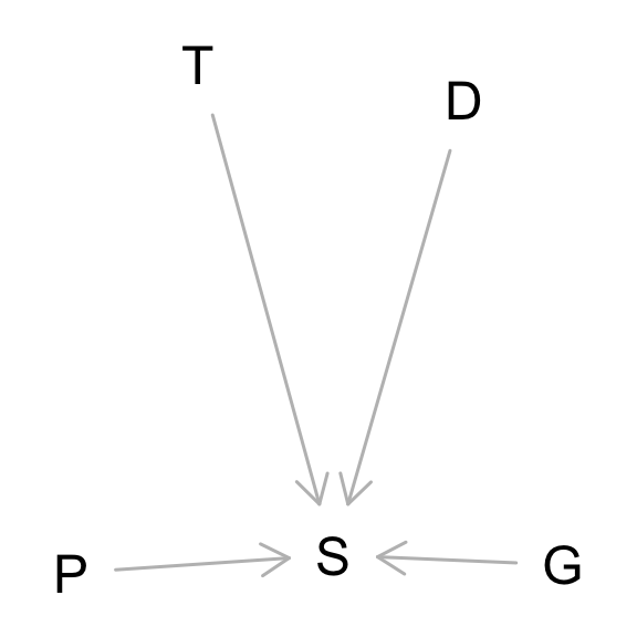
This is an experiment, so we know the treatments P, G, and D are not confounded. At least not in any obvious way. And then unobserved tank effects T also moderate the influence of the treatments. The model I used tries to estimate how P and G moderate one another. It ignores D, which we are allowed to do, because it is not a confound, just a competing cause. But I include tanks, which is also just a competing cause. Including competing causes helps with precision, if nothing else.
They just show inputs and outputs. To justify any particular statistical model, you need more than the DAG.
Question 3
Now estimate the causal effect of density on survival. Consider whether pred modifies the effect of density. There are several good ways to include density in your Binomial GLM. You could treat it as a continuous regression variable (possibly standardized). Or you could convert it to an ordered category (with three levels).
Compare the \(\sigma\) (tank standard deviation) posterior distribution to \(\sigma\) from your model in Problem 2. How are they different? Why?
Density is an important factor in these experiments. So let’s include it finally. I will do something simple, just include it as an additive effect that interacts with predators. But I will use the logarithm of density, so that it has implied diminishing returns on the log-odds scale.
dat$Do <- standardize(log(d$density))

m3 <- ulam(
  alist(
    S ~ binomial( D , p ),
    logit(p) <- a[T] + b[P,G] + bD[P]*Do,
    a[T] ~ normal( 0 , sigma ),
    matrix[P,G]:b ~ normal( 0 , 1 ),
    bD[P] ~ normal(0,0.5),
    sigma ~ exponential( 1 )
  ), data=dat , chains=4 , cores=4 , log_lik=TRUE )
## Running MCMC with 4 parallel chains, with 1 thread(s) per chain...
##
## Chain 1 Iteration:   1 / 1000 [  0%]  (Warmup)
## Chain 1 Iteration: 100 / 1000 [ 10%]  (Warmup)
## Chain 1 Iteration: 200 / 1000 [ 20%]  (Warmup)
## Chain 1 Iteration: 300 / 1000 [ 30%]  (Warmup)
## Chain 1 Iteration: 400 / 1000 [ 40%]  (Warmup)
## Chain 1 Iteration: 500 / 1000 [ 50%]  (Warmup)
## Chain 1 Iteration: 501 / 1000 [ 50%]  (Sampling)
## Chain 1 Iteration: 600 / 1000 [ 60%]  (Sampling)
## Chain 1 Iteration: 700 / 1000 [ 70%]  (Sampling)
## Chain 1 Iteration: 800 / 1000 [ 80%]  (Sampling)
## Chain 1 Iteration: 900 / 1000 [ 90%]  (Sampling)
## Chain 1 Iteration: 1000 / 1000 [100%]  (Sampling)
## Chain 2 Iteration:   1 / 1000 [  0%]  (Warmup)
## Chain 2 Iteration: 100 / 1000 [ 10%]  (Warmup)
## Chain 2 Iteration: 200 / 1000 [ 20%]  (Warmup)
## Chain 2 Iteration: 300 / 1000 [ 30%]  (Warmup)
## Chain 2 Iteration: 400 / 1000 [ 40%]  (Warmup)
## Chain 2 Iteration: 500 / 1000 [ 50%]  (Warmup)
## Chain 2 Iteration: 501 / 1000 [ 50%]  (Sampling)
## Chain 2 Iteration: 600 / 1000 [ 60%]  (Sampling)
## Chain 2 Iteration: 700 / 1000 [ 70%]  (Sampling)
## Chain 2 Iteration: 800 / 1000 [ 80%]  (Sampling)
## Chain 2 Iteration: 900 / 1000 [ 90%]  (Sampling)
## Chain 2 Iteration: 1000 / 1000 [100%]  (Sampling)
## Chain 3 Iteration:   1 / 1000 [  0%]  (Warmup)
## Chain 3 Iteration: 100 / 1000 [ 10%]  (Warmup)
## Chain 3 Iteration: 200 / 1000 [ 20%]  (Warmup)
## Chain 3 Iteration: 300 / 1000 [ 30%]  (Warmup)
## Chain 3 Iteration: 400 / 1000 [ 40%]  (Warmup)
## Chain 3 Iteration: 500 / 1000 [ 50%]  (Warmup)
## Chain 3 Iteration: 501 / 1000 [ 50%]  (Sampling)
## Chain 3 Iteration: 600 / 1000 [ 60%]  (Sampling)
## Chain 3 Iteration: 700 / 1000 [ 70%]  (Sampling)
## Chain 3 Iteration: 800 / 1000 [ 80%]  (Sampling)
## Chain 3 Iteration: 900 / 1000 [ 90%]  (Sampling)
## Chain 3 Iteration: 1000 / 1000 [100%]  (Sampling)
## Chain 4 Iteration:   1 / 1000 [  0%]  (Warmup)
## Chain 4 Iteration: 100 / 1000 [ 10%]  (Warmup)
## Chain 4 Iteration: 200 / 1000 [ 20%]  (Warmup)
## Chain 4 Iteration: 300 / 1000 [ 30%]  (Warmup)
## Chain 4 Iteration: 400 / 1000 [ 40%]  (Warmup)
## Chain 4 Iteration: 500 / 1000 [ 50%]  (Warmup)
## Chain 4 Iteration: 501 / 1000 [ 50%]  (Sampling)
## Chain 4 Iteration: 600 / 1000 [ 60%]  (Sampling)
## Chain 4 Iteration: 700 / 1000 [ 70%]  (Sampling)
## Chain 1 finished in 0.2 seconds.
## Chain 2 finished in 0.2 seconds.
## Chain 3 finished in 0.1 seconds.
## Chain 4 Iteration: 800 / 1000 [ 80%]  (Sampling)
## Chain 4 Iteration: 900 / 1000 [ 90%]  (Sampling)
## Chain 4 Iteration: 1000 / 1000 [100%]  (Sampling)
## Chain 4 finished in 0.1 seconds.
##
## All 4 chains finished successfully.
## Mean chain execution time: 0.2 seconds.
## Total execution time: 0.4 seconds.
precis(m3,3,pars=c("b","bD","sigma"))
##              mean        sd       5.5%      94.5%     n_eff     Rhat4
## b[1,1]  2.3473727 0.2911915  1.9004836  2.8429358 1324.4498 1.0033966
## b[1,2]  2.4927055 0.2976433  2.0269645  2.9834016 1707.5013 1.0001058
## b[2,1]  0.5257347 0.2236003  0.1769636  0.8770541  867.3344 1.0001885
## b[2,2] -0.3549865 0.2323851 -0.7201052  0.0147492 1013.5865 1.0027122
## bD[1]   0.1393125 0.2144765 -0.2121929  0.4681566 1602.1237 0.9997855
## bD[2]  -0.4715676 0.1742109 -0.7566293 -0.1871588 1129.7075 0.9993428
## sigma   0.6343169 0.1316046  0.4395601  0.8521297  381.6673 1.0113039
Again an interaction. Higher densities are worse for survival, but only in the presence of predators. The other estimates are not changed much. The \(\sigma\) estimate here is a little smaller than in the previous problem. This is just because density is an real cause of survival, so it explains some of the variation that was previously soaked up by tanks with different densities.