Problem Set 5 Solutions
This problem set is due on March 14, 2022 at 11:59am.
Question 1
Revisit the marriage, age, and happiness collider bias example from Chapter 6. Run models m6.9 and m6.10 again (pages 178–179). Compare these two models using both PSIS and WAIC. Which model is expected to make better predictions, according to these criteria? On the basis of the causal model, how should you interpret the parameter estimates from the model preferred by PSIS and WAIC?
library(rethinking)
d <- sim_happiness( seed=1977 , N_years=1000 )
precis(d)
##                   mean        sd      5.5%     94.5%     histogram
## age       3.300000e+01 18.768883  4.000000 62.000000 ▇▇▇▇▇▇▇▇▇▇▇▇▇
## married   3.007692e-01  0.458769  0.000000  1.000000    ▇▁▁▁▁▁▁▁▁▃
## happiness 6.832142e-19  1.214421 -1.789474  1.789474      ▇▅▇▅▅▇▅▇
## R code 6.22
d2 <- d[ d$age>17 , ] # only adults
d2$A <- ( d2$age - 18 ) / ( 65 - 18 )

## R code 6.23
d2$mid <- d2$married + 1
m6.9 <- quap(
    alist(
        happiness ~ dnorm( mu , sigma ),
        mu <- a[mid] + bA*A,
        a[mid] ~ dnorm( 0 , 1 ),
        bA ~ dnorm( 0 , 2 ),
        sigma ~ dexp(1)
    ) , data=d2 )

## R code 6.24
m6.10 <- quap(
    alist(
        happiness ~ dnorm( mu , sigma ),
        mu <- a + bA*A,
        a ~ dnorm( 0 , 1 ),
        bA ~ dnorm( 0 , 2 ),
        sigma ~ dexp(1)
    ) , data=d2 )
Model m6.9 contains both marriage status and age. Model m6.10 contains only age. Model m6.9 produces a confounded inference about the relationship between age and happiness, due to opening a collider path. To compare these models using PSIS and WAIC:
compare( m6.9 , m6.10 , func=PSIS )
##           PSIS       SE   dPSIS      dSE    pPSIS       weight
## m6.9  2713.996 37.56527   0.000       NA 3.751076 1.000000e+00
## m6.10 3101.925 27.75875 387.929 35.40121 2.350136 5.784794e-85
compare( m6.9 , m6.10 , func=WAIC )
##           WAIC       SE    dWAIC      dSE    pWAIC       weight
## m6.9  2714.256 37.51051   0.0000       NA 3.861509 1.000000e+00
## m6.10 3101.883 27.68399 387.6271 35.34372 2.328445 6.727359e-85
The model that produces the invalid inference, m6.9, is expected to predict much better. And it would. This is because the collider path does convey actual association. We simply end up mistaken about the causal inference. We should not use PSIS or WAIC to choose among models, unless we have some clear sense of the causal model. These criteria will happily favor confounded models.
So what about the coefficients in the confounded model?
precis( m6.9 , depth=2 )
##             mean         sd       5.5%      94.5%
## a[1]  -0.2350877 0.06348986 -0.3365568 -0.1336186
## a[2]   1.2585517 0.08495989  1.1227694  1.3943340
## bA    -0.7490274 0.11320112 -0.9299447 -0.5681102
## sigma  0.9897080 0.02255800  0.9536559  1.0257600
We cannot interpret these estimates without reference to the causal model.
Okay, you know that the bA parameter is bias by the collider relationship. This model suffers from collider bias, and so bA is not anything but a conditional association. It isn’t any kind of causal effect. The parameters a[1] and a[2] are intercepts for unmarried and married, respectively. But do they correctly estimate the effect of marriage on happiness? No, because marriage in this example does not influence happiness. It is a consequence of happiness.
So what do they estimate? They measure the association between marriage and happiness. But they do it with bias, because the model also includes age. To prove this to yourself, fit a model that stratifies happiness by marriage status but ignore age. You’ll see that the a[1] and a[2] estimates you get are different, once you omit age from the model. In sum, every parameter in the model is a non-causal association.
Question 2
Reconsider the urban fox analysis from last week’s homework. On the basis of PSIS and WAIC scores, which combination of variables best predicts body weight (W, weight)? How would you interpret the estimates from the best scoring model?
library(rethinking)
data(foxes)
d <- foxes
d$W <- standardize(d$weight)
d$A <- standardize(d$area)
d$F <- standardize(d$avgfood)
d$G <- standardize(d$groupsize)

tau <- 0.5

m1 <- quap(
    alist(
        W ~ dnorm( mu , sigma ),
        mu <- a + bF*F + bG*G + bA*A,
        a ~ dnorm(0,0.2),
        c(bF,bG,bA) ~ dnorm(0,tau),
        sigma ~ dexp(1)
    ), data=d )

m2 <- quap(
    alist(
        W ~ dnorm( mu , sigma ),
        mu <- a + bF*F + bG*G,
        a ~ dnorm(0,0.2),
        c(bF,bG) ~ dnorm(0,tau),
        sigma ~ dexp(1)
    ), data=d )

m3 <- quap(
    alist(
        W ~ dnorm( mu , sigma ),
        mu <- a + bG*G + bA*A,
        a ~ dnorm(0,0.2),
        c(bG,bA) ~ dnorm(0,tau),
        sigma ~ dexp(1)
    ), data=d )

m4 <- quap(
    alist(
        W ~ dnorm( mu , sigma ),
        mu <- a + bF*F,
        a ~ dnorm(0,0.2),
        bF ~ dnorm(0,tau),
        sigma ~ dexp(1)
    ), data=d )

m5 <- quap(
    alist(
        W ~ dnorm( mu , sigma ),
        mu <- a + bA*A,
        a ~ dnorm(0,0.2),
        bA ~ dnorm(0,tau),
        sigma ~ dexp(1)
), data=d )

compare( m1 , m2 , m3 , m4 , m5 , func=PSIS )
##        PSIS       SE      dPSIS      dSE    pPSIS      weight
## m1 323.6575 16.52470  0.0000000       NA 5.054023 0.355981305
## m3 323.7961 15.85058  0.1386364 3.138860 3.668507 0.332141140
## m2 323.9523 16.14808  0.2948093 3.403063 3.713715 0.307192193
## m4 333.4974 13.90059  9.8399008 7.315596 2.445553 0.002598483
## m5 333.9359 13.96706 10.2784170 7.382642 2.728767 0.002086879
So the model with all three predictors is very slightly better than the model with only F and G. See the DAG from Problem Set 4 for original DAG.
precis(m1)
##                mean         sd         5.5%      94.5%
## a     -1.083245e-05 0.07936248 -0.126847405  0.1268257
## bF     2.968635e-01 0.20960154 -0.038120245  0.6318472
## bG    -6.396302e-01 0.18161573 -0.929887233 -0.3493732
## bA     2.782728e-01 0.17011319  0.006399093  0.5501466
## sigma  9.312129e-01 0.06100115  0.833721292  1.0287045
We don’t know the true causal effects in this example. The goal is just to use the DAG to reason what these coefficients are estimating, if anything.
First consider F and bF. Since G is in the model, the indirect causal effect of F on W is missing. So bF only measures the direct path. But it doesn’t even do that completely, because A is also in the model. You saw in an earlier lecture that including a cause of the exposure is usually a bad idea, because it statistical reduces variation in the exposure. So bF is probably less accurate than if we omitted A. But it estimates the direct causal effect of F on W. Second consider G. bG estimates the direct effect of G on W.
Now what about A? This is a weird one. From the perspective of A, including its mediator F should block all of its association with W. So it isn’t a measure of anything, but it is a kind of test of test of the DAG structure.
There may be unobserved confounding or more causal paths that explain why A and W remain associated even after stratifying by F. However, since the model without A has almost the same PSIS score as the one with it, maybe there isn’t much statistical support for A being associated with W here anyway. A regression that includes only A and F shows no association really between A and W. Why does including G strength the association between A and W? It could just be a fluke of the sample, or it could indicate something is wrong with the causal structure.
Optional Question (Not Graded)
Build a predictive model of the relationship show on the cover of the book, the relationship between the timing of cherry blossoms and March temperature in the same year. The data are found in data(cherry_blossoms). Consider at least two functions to predict doy with temp. Compare them with PSIS or WAIC.
Suppose March temperatures reach 9 degrees by the year 2050. What does your best model predict for the predictive distribution of the day-in-year that the cherry trees will blossom?
Start by preparing the data. In this sample, you need to drop the cases with missing values, and that may catch you by surprise.
data(cherry_blossoms)
d <- cherry_blossoms

d$D <- standardize(d$doy)
d$T <- standardize(d$temp)

dd <- d[ complete.cases(d$D,d$T) , ]

m3a <- ulam(
    alist(
        D ~ dnorm(mu,sigma),
        mu <- a,
        a ~ dnorm(0,10),
        sigma ~ dexp(1)
    ) , data=list(D=dd$D,T=dd$T), log_lik = TRUE )
## Running MCMC with 1 chain, with 1 thread(s) per chain...
##
## Chain 1 Iteration:   1 / 1000 [  0%]  (Warmup)
## Chain 1 Iteration: 100 / 1000 [ 10%]  (Warmup)
## Chain 1 Iteration: 200 / 1000 [ 20%]  (Warmup)
## Chain 1 Iteration: 300 / 1000 [ 30%]  (Warmup)
## Chain 1 Iteration: 400 / 1000 [ 40%]  (Warmup)
## Chain 1 Iteration: 500 / 1000 [ 50%]  (Warmup)
## Chain 1 Iteration: 501 / 1000 [ 50%]  (Sampling)
## Chain 1 Iteration: 600 / 1000 [ 60%]  (Sampling)
## Chain 1 Iteration: 700 / 1000 [ 70%]  (Sampling)
## Chain 1 Iteration: 800 / 1000 [ 80%]  (Sampling)
## Chain 1 Iteration: 900 / 1000 [ 90%]  (Sampling)
## Chain 1 Iteration: 1000 / 1000 [100%]  (Sampling)
## Chain 1 finished in 0.2 seconds.
m3b <- ulam(
    alist(
        D ~ dnorm(mu,sigma),
        mu <- a + b*T,
        a ~ dnorm(0,10),
        b ~ dnorm(0,10),
        sigma ~ dexp(1)
    ) , data=list(D=dd$D,T=dd$T), log_lik = TRUE )
## Running MCMC with 1 chain, with 1 thread(s) per chain...
##
## Chain 1 Iteration:   1 / 1000 [  0%]  (Warmup)
## Chain 1 Iteration: 100 / 1000 [ 10%]  (Warmup)
## Chain 1 Iteration: 200 / 1000 [ 20%]  (Warmup)
## Chain 1 Iteration: 300 / 1000 [ 30%]  (Warmup)
## Chain 1 Iteration: 400 / 1000 [ 40%]  (Warmup)
## Chain 1 Iteration: 500 / 1000 [ 50%]  (Warmup)
## Chain 1 Iteration: 501 / 1000 [ 50%]  (Sampling)
## Chain 1 Iteration: 600 / 1000 [ 60%]  (Sampling)
## Chain 1 Iteration: 700 / 1000 [ 70%]  (Sampling)
## Chain 1 Iteration: 800 / 1000 [ 80%]  (Sampling)
## Chain 1 Iteration: 900 / 1000 [ 90%]  (Sampling)
## Chain 1 Iteration: 1000 / 1000 [100%]  (Sampling)
## Chain 1 finished in 0.5 seconds.
m3c <- ulam(
    alist(
        D ~ dnorm(mu,sigma),
        mu <- a + b1*T + b2*T^2,
        a ~ dnorm(0,10),
        c(b1,b2) ~ dnorm(0,10),
        sigma ~ dexp(1)
    ) , data=list(D=dd$D,T=dd$T), log_lik = TRUE )
## Running MCMC with 1 chain, with 1 thread(s) per chain...
##
## Chain 1 Iteration:   1 / 1000 [  0%]  (Warmup)
## Chain 1 Iteration: 100 / 1000 [ 10%]  (Warmup)
## Chain 1 Iteration: 200 / 1000 [ 20%]  (Warmup)
## Chain 1 Iteration: 300 / 1000 [ 30%]  (Warmup)
## Chain 1 Iteration: 400 / 1000 [ 40%]  (Warmup)
## Chain 1 Iteration: 500 / 1000 [ 50%]  (Warmup)
## Chain 1 Iteration: 501 / 1000 [ 50%]  (Sampling)
## Chain 1 Iteration: 600 / 1000 [ 60%]  (Sampling)
## Chain 1 Iteration: 700 / 1000 [ 70%]  (Sampling)
## Chain 1 Iteration: 800 / 1000 [ 80%]  (Sampling)
## Chain 1 Iteration: 900 / 1000 [ 90%]  (Sampling)
## Chain 1 Iteration: 1000 / 1000 [100%]  (Sampling)
## Chain 1 finished in 0.6 seconds.
compare( m3a , m3b , m3c , func=PSIS )
##         PSIS       SE     dPSIS        dSE    pPSIS       weight
## m3b 2112.628 40.69893  0.000000         NA 3.052989 6.897909e-01
## m3c 2114.226 40.69915  1.598284  0.2708888 3.726015 3.102091e-01
## m3a 2199.324 39.35050 86.696434 16.6809424 1.987350 1.029974e-19
The linear m3b is slightly better than m3c. Both are much better than the intercept-only m3a. Now we need to generate a predictive distribution for the first day of bloom. We do this by simulating from the model for a specific temperature. The only trick here is to remember that both the predictor and outcome were standardized above. If you didn’t standardized, then you won’t need to convert back. But my code below does.
# predict

Tval <- (9 - mean(d$temp,na.rm=TRUE))/sd(d$temp,na.rm=TRUE)
D_sim <- sim( m3b , data=list(T=Tval) )
# put back on natural scale
doy_sim <- D_sim*sd(d$doy,na.rm=TRUE) + mean(d$doy,na.rm=TRUE)
dens( doy_sim , lwd=4 , col=2 , xlab="day in year 1st bloom")
abline(v=89,lty=1)
dens( d$doy , add=TRUE , lwd=3 )
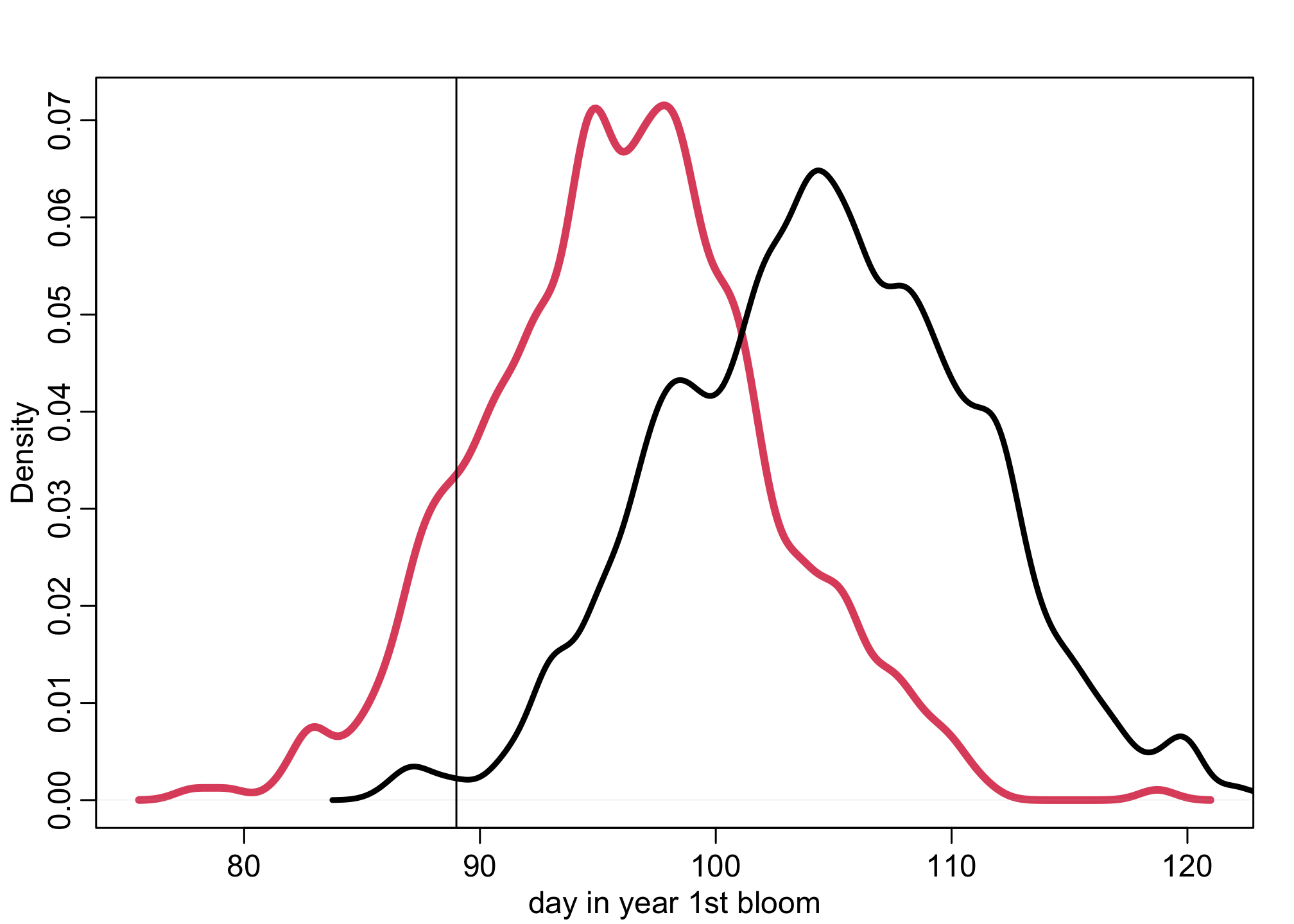
The red density is the predictive distribution for 9 degrees. The black density is the observed historical data. The vertical line is April 1. This is a linear projection, so it is reasonable to question whether such a large degree of continued warming would continue to exert a linear effect on timing of the blossoms. But so far the effect has been quite linear. To do better, we’d need to use some more science, not just statistics.