Problem Set 4 Solutions
This problem set is due on February 28, 2022 at 11:59am.
%60%22%0A---%0A%0AThis problem set is due on February 28, 2022 at 11:59am.%0A%0A- **Name**:%0A- **UNCC ID**: %0A- **Other student worked with (optional)**:%0A%0A%23%23 Question 1%0A%0AThe first two problems are based on the same data. The data in %60data(foxes)%60 are 116 foxes from 30 different urban groups in England. %0A%0A%60%60%60%7Br warning=FALSE,message=FALSE%7D%0Alibrary(rethinking)%0Adata(foxes)%0Ad%3C- foxes%0Ahead(d)%0A%60%60%60%0A%0AThese fox groups are like street gangs. Group size (%60groupsize%60) varies from 2 to 8 individuals. Each group maintains its own (almost exclusive) urban territory. Some territories are larger than others. The %60area%60 variable encodes this information. Some territories also have more %60avgfood%60 than others. And food influences the %60weight%60 of each fox. Assume this DAG:%0A%0A%60%60%60%7Br fig.height=4, fig.width=4%7D%0Alibrary(dagitty)%0A%0Ag %3C- dagitty('dag %7B%0Abb=%220,0,1,1%22%0AA %5Bpos=%220.450,0.290%22%5D%0AF %5Bexposure,pos=%220.333,0.490%22%5D%0AG %5Bpos=%220.539,0.495%22%5D%0AW %5Boutcome,pos=%220.445,0.686%22%5D%0AA -%3E F%0AF -%3E G%0AF -%3E W%0AG -%3E W%0A%7D%0A%0A')%0Aplot(g)%0A%60%60%60%0A%0Awhere F is %60avgfood%60, G is %60groupsize%60, A is %60area%60, and W is %60weight%60.%0A%0A**Part 1**: Use the backdoor criterion and estimate the total causal influence of A on F. %0A%0A%60%60%60%7Br eval=FALSE, include=FALSE%7D%0A%23 type in your code here%0A%0A%60%60%60%0A%0A**Part 2**: What effect would increasing the area of a territory have on the amount of food inside it?%0A%0A%5BWrite answer here in sentences%5D%0A%0A%23%23 Question 2%0A%0ANow infer both the **total** and **direct** causal effects of adding food F to a territory on the weight W of foxes. Which covariates do you need to adjust for in each case? In light of your estimates from this problem and the previous one, what do you think is going on with these foxes? Feel free to speculate%E2%80%94all that matters is that you justify your speculation.%0A%0A%0A%0A%60%60%60%7Br eval=FALSE, include=FALSE%7D%0A%23 Total causal effect: type in your code here%0A%0A%60%60%60%0A%0A%0A%0A%60%60%60%7Br eval=FALSE, include=FALSE%7D%0A%23 For the direct causal effect: type in your code here%0A%0A%60%60%60%0A%0A%23%23 Question 3%0A%0AReconsider the Table 2 Fallacy example (from Lecture 6), this time with an unobserved confound U that influences both smoking S and stroke Y. Here%E2%80%99s the modified DAG:%0A%0A%60%60%60%7Br echo=FALSE, out.width = '50%25'%7D%0A%23 run this chunk to view the image%0Aknitr::include_graphics(%22https://raw.githubusercontent.com/wesslen/dsba6010-spring2022/master/static/img/assignments/04-problem-set/04-problem-set-0.png%22)%0A%60%60%60%0A%0APart 1: use the backdoor criterion to determine an adjustment set that allows you to estimate the causal effect of X on Y, i.e. P(Y%7Cdo(X)). %0A%0AFor this exercise, you can use %5Bdagitty.net%5D(http://www.dagitty.net/dags.html).%0A%0AStep 1: Input your DAG into Dagitty.net and copy/paste your results here:%0A%0A%60%60%60%7Br eval=FALSE%7D%0A%23 insert code here%0A%0Ag %3C- dagitty('%0A %23 copy/paste dagitty.net code for DAG here%0A ')%0A%60%60%60%0A%0AStep 2: What is the adjustment set to estimate the causal effect of X on Y?%0A%0A%60%60%60%7Br eval=FALSE, include=FALSE%7D%0A%23 find adjustment set: type in your code here%0A%0A%60%60%60%0A%0APart 2: Explain the proper interpretation of each coefficient implied by the regression model that corresponds to the adjustment set. Which coefficients (slopes) are causal and which are not? There is no need to fit any models. Just think through the implications.%0A%0A%5BWrite answer here in sentences%5D)
Question 1
The first two problems are based on the same data. The data in data(foxes) are 116 foxes from 30 different urban groups in England.
library(rethinking)
data(foxes)
d<- foxes
head(d)
##   group avgfood groupsize area weight
## 1     1    0.37         2 1.09   5.02
## 2     1    0.37         2 1.09   2.84
## 3     2    0.53         2 2.05   5.33
## 4     2    0.53         2 2.05   6.07
## 5     3    0.49         2 2.12   5.85
## 6     3    0.49         2 2.12   3.25
These fox groups are like street gangs. Group size (groupsize) varies from 2 to 8 individuals. Each group maintains its own (almost exclusive) urban territory. Some territories are larger than others. The area variable encodes this information. Some territories also have more avgfood than others. And food influences the weight of each fox. Assume this DAG:
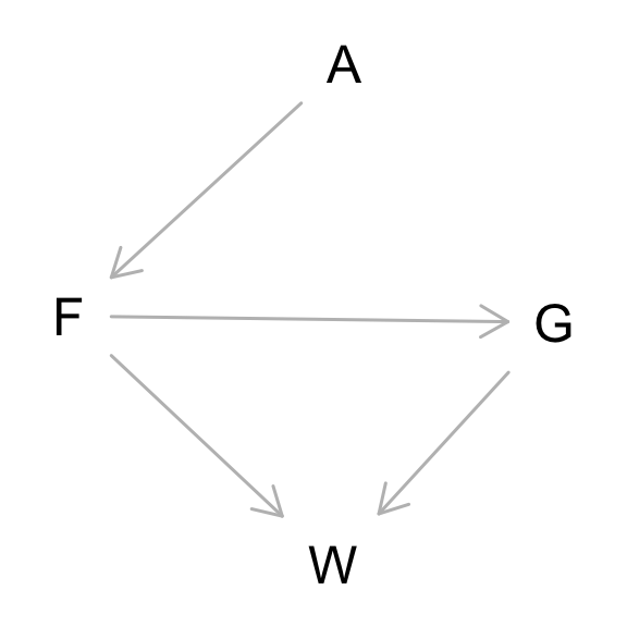
where F is avgfood, G is groupsize, A is area, and W is weight.
Part 1: Use the backdoor criterion and estimate the total causal influence of A on F.
library(rethinking)
data(foxes)
d<- foxes
head(d)
##   group avgfood groupsize area weight
## 1     1    0.37         2 1.09   5.02
## 2     1    0.37         2 1.09   2.84
## 3     2    0.53         2 2.05   5.33
## 4     2    0.53         2 2.05   6.07
## 5     3    0.49         2 2.12   5.85
## 6     3    0.49         2 2.12   3.25
d$W <- standardize(d$weight)
d$A <- standardize(d$area)
d$F <- standardize(d$avgfood)
d$G <- standardize(d$groupsize)

# 1

m1 <- quap(
    alist(
        F ~ dnorm( mu , sigma ),
        mu <- a + bA*A,
        a ~ dnorm(0,0.2),
        bA ~ dnorm(0,0.5),
        sigma ~ dexp(1)
    ), data=d )

precis(m1)
##                mean         sd        5.5%      94.5%
## a     -1.432375e-07 0.04231133 -0.06762181 0.06762153
## bA     8.764743e-01 0.04332411  0.80723402 0.94571462
## sigma  4.662604e-01 0.03052492  0.41747567 0.51504511
Part 2: What effect would increasing the area of a territory have on the amount of food inside it?
Territory size seems to have a substantial effect on food availability. These are standardized variables, so bA above means that each standard deviation change in area results on average in about 0.9 standard deviations of change in food availability.
Question 2
Now infer both the total and direct causal effects of adding food F to a territory on the weight W of foxes. Which covariates do you need to adjust for in each case? In light of your estimates from this problem and the previous one, what do you think is going on with these foxes? Feel free to speculate—all that matters is that you justify your speculation.
To infer the causal influence of avgfood on weight, we need to close any back-door paths. There are no back-door paths in the DAG. So again, just use a model with a single predictor
Total causal effect:
m2 <- quap(
    alist(
        W ~ dnorm( mu , sigma ),
        mu <- a + bF*F,
        a ~ dnorm(0,0.2),
        bF ~ dnorm(0,0.5),
        sigma ~ dexp(1)
    ), data=d )

precis(m2)
##                mean         sd       5.5%     94.5%
## a      1.116891e-06 0.08360032 -0.1336083 0.1336106
## bF    -2.420602e-02 0.09088521 -0.1694581 0.1210461
## sigma  9.911462e-01 0.06465894  0.8878087 1.0944836
There seems to be only a small total effect of food on weight, if there is any effect at all. It’s about equally plausible that it’s negative as positive, and it’s small either way
For the direct causal effect, we need to block the mediated path through group size G. That means stratify by group size.
m2b <- quap(
    alist(
        W ~ dnorm( mu , sigma ),
        mu <- a + bF*F + bG*G,
        a ~ dnorm(0,0.2),
        c(bF,bG) ~ dnorm(0,0.5),
        sigma ~ dexp(1)
    ), data=d )

precis(m2b)
##                mean         sd       5.5%      94.5%
## a      1.330174e-08 0.08013807 -0.1280761  0.1280761
## bF     4.772531e-01 0.17912322  0.1909796  0.7635266
## bG    -5.735257e-01 0.17914172 -0.8598288 -0.2872227
## sigma  9.420439e-01 0.06175255  0.8433514  1.0407364
The direct effect of food on weight is positive (0.19–0.76), it seems. That makes sense. This model also gives us the direct effect (also the total effect) of group size on weight. And it is the opposite and of the same magnitude as the direct effect of food. These two effects seem to cancel one another. That may be why the total effect of food is about zero: the direct effect is positive but the mediated effect through groups size is negative.
What is going on here? Larger territories increase available food (problem 1). But increases in food (and territory) do not influence fox weight. The reason seems to be because adding more food directly increases weight, but the path through group size cancels that increase. To check this idea, we can estimate the causal effect of food on groups size:
m2c <- quap(
    alist(
        G ~ dnorm( mu , sigma ),
        mu <- a + bF*F,
        a ~ dnorm(0,0.2),
        bF ~ dnorm(0,0.5),
        sigma ~ dexp(1)
    ), data=d )

precis(m2c)
##                mean         sd        5.5%      94.5%
## a     -8.680653e-09 0.03916832 -0.06259855 0.06259853
## bF     8.957170e-01 0.03999361  0.83179953 0.95963455
## sigma  4.301860e-01 0.02816911  0.38516637 0.47520572
Food appears to have a large and reliably (0.83–0.96) effect on group size. That is, more food means more foxes. This is consistent with the idea that the mediating influence of group size cancels the direct influence of more food on individual fox body weight. In simple terms, the benefits of more food are canceled by more foxes being attracted to the food, so each fox gets the same amount.
Question 3
Reconsider the Table 2 Fallacy example (from Lecture 6), this time with an unobserved confound U that influences both smoking S and stroke Y. Here’s the modified DAG:
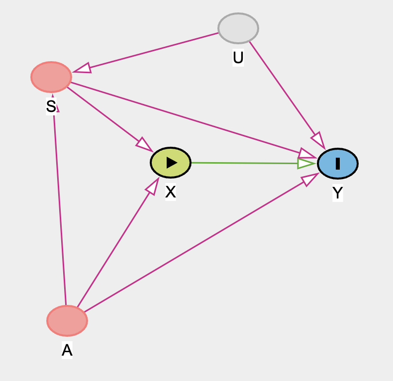
Part 1: use the backdoor criterion to determine an adjustment set that allows you to estimate the causal effect of X on Y, i.e. P(Y|do(X)).
For this exercise, you can use dagitty.net.
First, input your DAG into Dagitty.net and copy/paste your results here:
# insert code here

g <- dagitty('dag {
bb="0,0,1,1"
A [pos="0.318,0.698"]
S [pos="0.282,0.370"]
U [latent,pos="0.475,0.248"]
X [exposure,pos="0.430,0.470"]
Y [outcome,pos="0.581,0.465"]
A -> S
A -> X
A -> Y
S -> X
S -> Y
U -> S
U -> Y
X -> Y
}')
Next, find what is the adjustment set to estimate the causal effect of X on Y?
dagitty::adjustmentSets(g)
## { A, S }
Part 2: Explain the proper interpretation of each coefficient implied by the regression model that corresponds to the adjustment set. Which coefficients (slopes) are causal and which are not? There is no need to fit any models. Just think through the implications.
Now the implications for each coefficient. The coefficient for X should still be the estimate of the causal effect of X on Y, P(Y|do(X)). But the other coefficients are now biased by U. When we stratify by S, we open the collider path that S is on: A → S ← U. Now the coefficients for A and S are not even partial causal effects, because both are biased by the collider through U. In effect the unobserved confound makes the control coefficients uninterpretable even as partial causal effects.
The irony here is that is still possible to estimate the casual effect of age A on Y. But in the model that stratifies by S, the coefficient for age becomes confounded. It really is not safe to interpret control coefficients, unless there is an explicit causal model.
Package versions
sessionInfo()
## R version 4.1.1 (2021-08-10)
## Platform: aarch64-apple-darwin20 (64-bit)
## Running under: macOS Monterey 12.1
##
## Matrix products: default
## BLAS:   /Library/Frameworks/R.framework/Versions/4.1-arm64/Resources/lib/libRblas.0.dylib
## LAPACK: /Library/Frameworks/R.framework/Versions/4.1-arm64/Resources/lib/libRlapack.dylib
##
## locale:
## [1] en_US.UTF-8/en_US.UTF-8/en_US.UTF-8/C/en_US.UTF-8/en_US.UTF-8
##
## attached base packages:
## [1] parallel  stats     graphics  grDevices datasets  utils     methods
## [8] base
##
## other attached packages:
## [1] dagitty_0.3-1        rethinking_2.21      cmdstanr_0.4.0.9001
## [4] rstan_2.21.3         ggplot2_3.3.5        StanHeaders_2.21.0-7
##
## loaded via a namespace (and not attached):
##  [1] sass_0.4.0           jsonlite_1.7.2       bslib_0.3.1
##  [4] RcppParallel_5.1.4   assertthat_0.2.1     posterior_1.1.0
##  [7] distributional_0.2.2 highr_0.9            stats4_4.1.1
## [10] tensorA_0.36.2       renv_0.14.0          yaml_2.2.1
## [13] pillar_1.6.4         backports_1.4.1      lattice_0.20-44
## [16] glue_1.6.0           uuid_1.0-3           digest_0.6.29
## [19] checkmate_2.0.0      colorspace_2.0-2     htmltools_0.5.2
## [22] pkgconfig_2.0.3      bookdown_0.24        purrr_0.3.4
## [25] mvtnorm_1.1-3        scales_1.1.1         processx_3.5.2
## [28] tibble_3.1.6         generics_0.1.1       farver_2.1.0
## [31] ellipsis_0.3.2       withr_2.4.3          cli_3.1.0
## [34] mime_0.12            magrittr_2.0.1       crayon_1.4.2
## [37] evaluate_0.14        ps_1.6.0             fs_1.5.0
## [40] fansi_0.5.0          MASS_7.3-54          pkgbuild_1.3.1
## [43] blogdown_1.5         tools_4.1.1          loo_2.4.1
## [46] prettyunits_1.1.1    lifecycle_1.0.1      matrixStats_0.61.0
## [49] stringr_1.4.0        V8_3.6.0             munsell_0.5.0
## [52] callr_3.7.0          compiler_4.1.1       jquerylib_0.1.4
## [55] rlang_0.4.12         grid_4.1.1           rstudioapi_0.13
## [58] base64enc_0.1-3      rmarkdown_2.11       boot_1.3-28
## [61] xaringanExtra_0.5.5  gtable_0.3.0         codetools_0.2-18
## [64] curl_4.3.2           inline_0.3.19        abind_1.4-5
## [67] DBI_1.1.1            R6_2.5.1             gridExtra_2.3
## [70] lubridate_1.8.0      knitr_1.36           dplyr_1.0.7
## [73] fastmap_1.1.0        utf8_1.2.2           downloadthis_0.2.1
## [76] bsplus_0.1.3         shape_1.4.6          stringi_1.7.6
## [79] Rcpp_1.0.7           vctrs_0.3.8          tidyselect_1.1.1
## [82] xfun_0.28            coda_0.19-4