Problem Set 3 Solutions
This problem set is due on February 21, 2022 at 11:59am.
Question 1
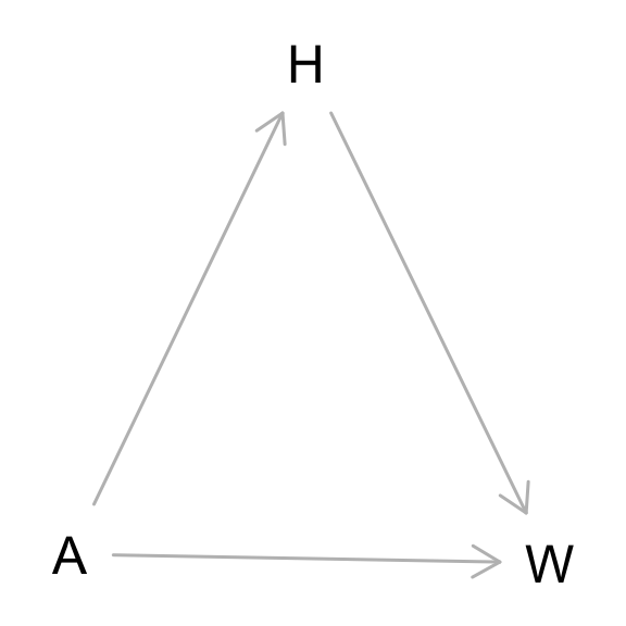
From the Howell1 dataset, consider only the people younger than 13 years old. Estimate the causal association between age and weight. Assume that age influences weight through two paths. First, age influences height, and height influences weight. Second, age directly influences weight through age related changes in muscle growth and body proportions. All of this implies this causal model (DAG):
library(dagitty)

g <- dagitty('dag {
bb="0,0,1,1"
A [pos="0.251,0.481"]
H [pos="0.350,0.312"]
W [pos="0.452,0.484"]
A -> H
A -> W
H -> W
}
')
plot(g)
Use a linear regression to estimate the total (not just direct) causal effect of each year of growth on weight. Be sure to carefully consider the priors. Try using prior predictive simulation to assess what they imply.
library(rethinking)
data(Howell1)
d <- Howell1
d <- d[ d$age < 13 , ]

# sim from priors
n <- 10
a <- rnorm(n,5,1)
b <- rlnorm(n,0,1)
# blank(bty="n")
plot( NULL , xlim=range(d$age) , ylim=range(d$weight), xlab="age", ylab="weight" )
for ( i in 1:n ) abline( a[i] , b[i] , lwd=3 , col=2 )
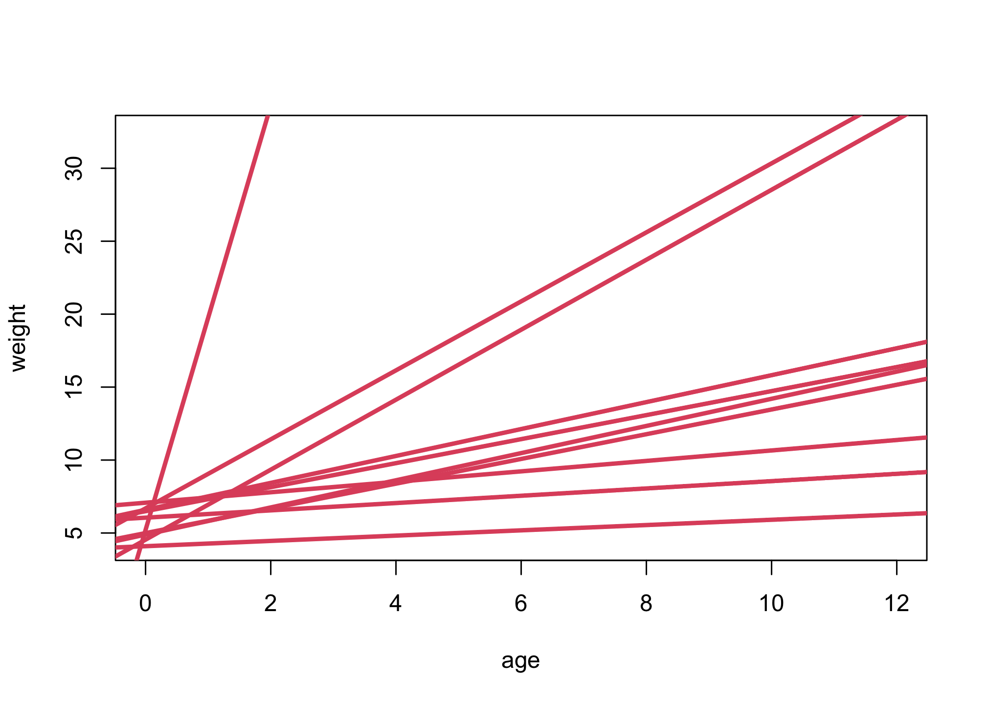
These are guesses that include that the relationship must be positive and that weight at age zero is birth weight, an average around 5 kg.
m2 <- quap(
    alist(
        W ~ dnorm( mu , sigma ),
        mu <- a + b*A,
        a ~ dnorm(5,1),
        b ~ dlnorm(0,1),
        sigma ~ dexp(1)
    ), data=list(W=d$weight,A=d$age) )

precis(m2)
##           mean         sd     5.5%    94.5%
## a     7.179132 0.33980549 6.636057 7.722206
## b     1.373792 0.05243257 1.289995 1.457589
## sigma 2.507394 0.14535422 2.275090 2.739698
The causal effect of each year of growth is given by the parameter b, so its 89% interval is 1.29 to 1.46 kg / year.
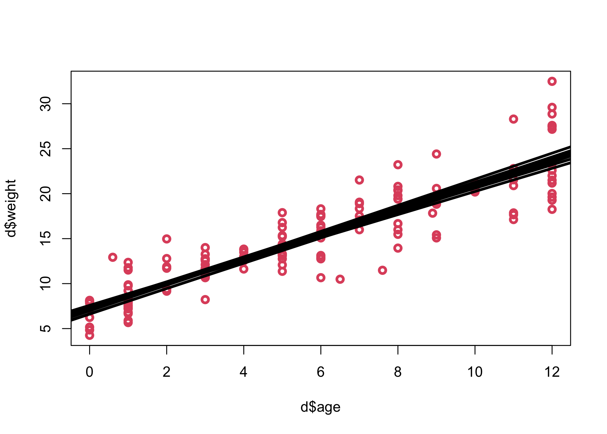
Let’s first look at the means.
# approach 1: use extract.samples
plot( d$age , d$weight , lwd=3, col=2 )
post <- extract.samples(m2)
for ( i in 1:10 ) abline( post$a[i] , post$b[i] , lwd=3 , col=1 )
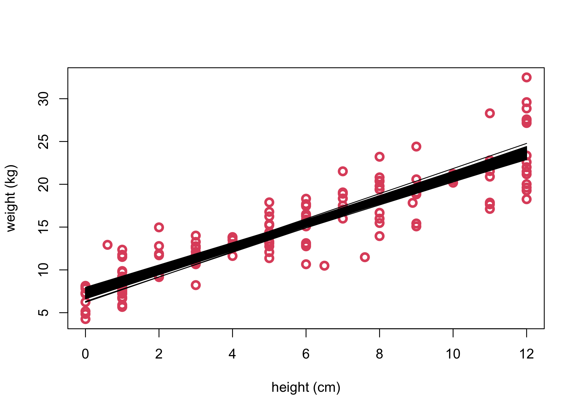
# approach 2: use link function
sim_n=100

xseq <- seq(from=0,to=12,by=1)
mu <- link(m2,data=list( A=xseq), sim_n)
mu.mean <- apply( mu , 2 , mean )

plot(d$age, d$weight, col=2 , lwd=3,
     cex=1.2, xlab="height (cm)", ylab="weight (kg)")
for ( i in 1:sim_n )
    lines( xseq , mu[i,] , pch=16, col=1 )
Question 2
Now suppose the causal association between age and weight might be different for boys and girls. Use a single linear regression, with a categorical variable for sex, to estimate the total causal effect of age on weight separately for boys and girls. How do girls and boys differ? Provide one or more posterior contrasts as a summary.
library(rethinking)
data(Howell1)
d <- Howell1
d <- d[ d$age < 13 , ]

dat <- list(W=d$weight,A=d$age,S=d$male+1)

m3 <- quap(
    alist(
        W ~ dnorm( mu , sigma ),
        mu <- a[S] + b[S]*A,
        a[S] ~ dnorm(5,1),
        b[S] ~ dlnorm(0,1),
        sigma ~ dexp(1)
    ), data=dat )

# blank(bty="n")
plot( d$age , d$weight , lwd=3, col=ifelse(d$male==1,4,2) , xlab="age (years)" , ylab="weight (kg)" )
Aseq <- 0:12

# girls
muF <- link(m3,data=list(A=Aseq,S=rep(1,13)))
shade( apply(muF,2,PI,0.99) , Aseq , col=col.alpha(2,0.5) )
lines( Aseq , apply(muF,2,mean) , lwd=3 , col=2 )

# boys
muM <- link(m3,data=list(A=Aseq,S=rep(2,13)))
shade( apply(muM,2,PI,0.99) , Aseq , col=col.alpha(4,0.5) )
lines( Aseq , apply(muM,2,mean) , lwd=3 , col=4 )
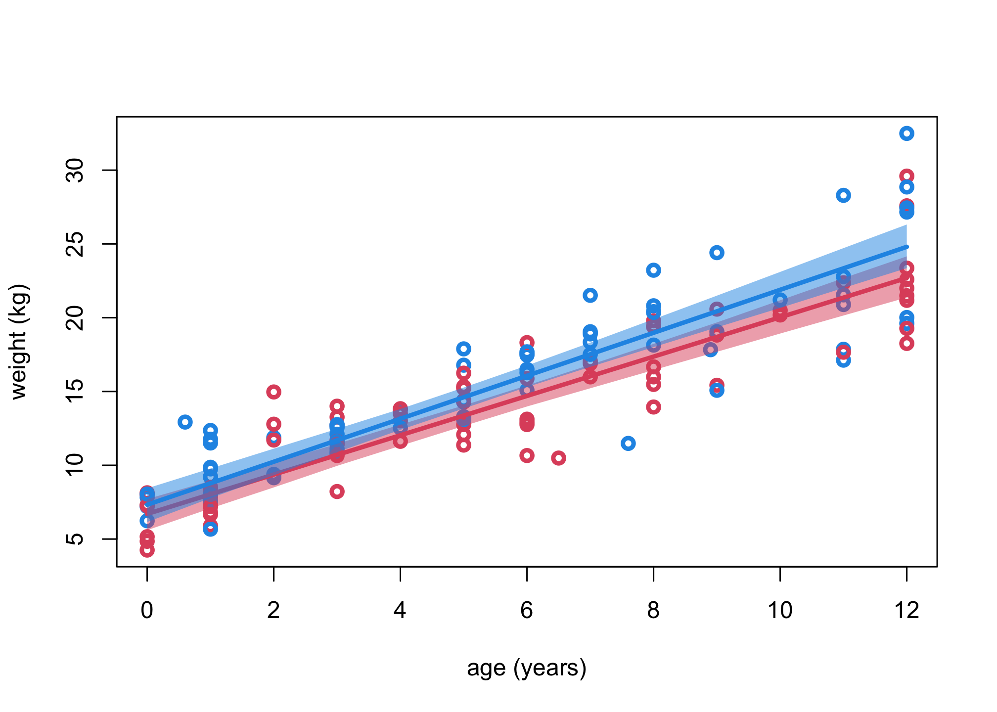
So boys look a little heavier than girls at all ages and seem to increase slightly faster as well. Let’s do a posterior contrast across ages though, so we can get make sure.
N_sim = 100

Aseq <- 0:12
mu1 <- sim(m3,data=list(A=Aseq,S=rep(1,13)), N_sim)
mu2 <- sim(m3,data=list(A=Aseq,S=rep(2,13)), N_sim)
mu_contrast <- mu1
for ( i in 1:13 ) mu_contrast[,i] <- mu2[,i] - mu1[,i]
plot( NULL , xlim=c(0,13) , ylim=c(-15,15) , xlab="age" , ylab="weight difference (boys-girls)" )

for ( p in c(0.5,0.67,0.89,0.99) )
shade( apply(mu_contrast,2,PI,prob=p) , Aseq )

abline(h=0,lty=2,lwd=2)

for ( i in 1:13 ) points( rep(i-1,N_sim), mu_contrast[1:N_sim,i] , col=ifelse(mu_contrast[1:N_sim,i]>0,4,2) , lwd=3 )
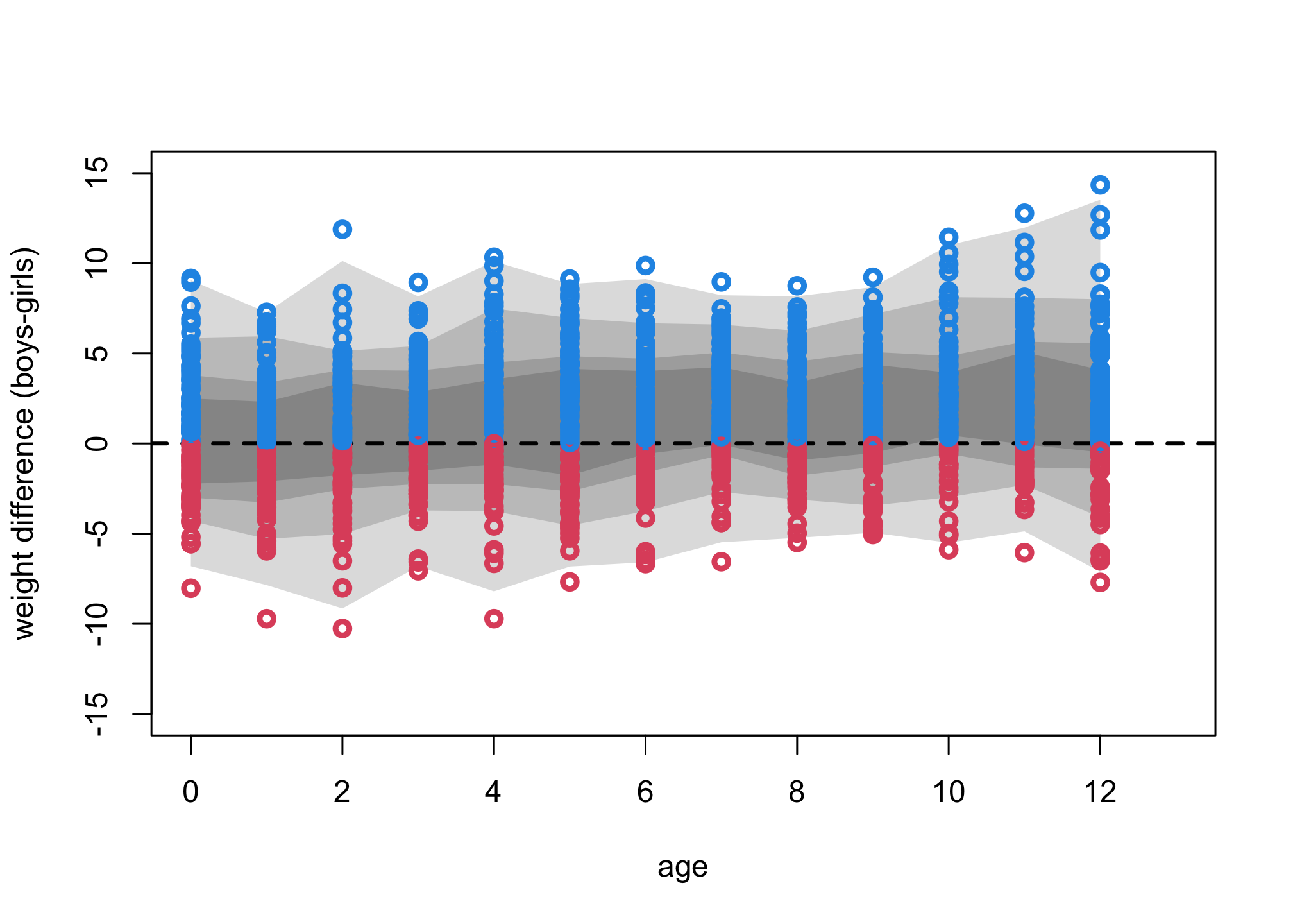
These contrasts use the entire weight distribution, not just the expectations. Boys do tend to be heavier than girls at all ages, but the distributions overlap a lot. The difference increases with age. This is good moment to repeat Richard’s sermon on zero. The fact that these contrasts all overlap zero is no reason to assert that there is no difference in weight between boys and girls. That would be silly. But that is exactly what researchers do every time they look if an interval overlaps zero and then act as if the estimate was exactly zero.
Question 3
For this problem, we want to compare the difference between Frequentist and Bayesian linear regressions. We’re going to use the similar functions from section 4.5.
To begin, run the same code to get the model m4.5 (i.e., run R code 4.65).
# R code 4.65 + 4.66 (precis)
library(rethinking)
data(Howell1)
d <- Howell1
d$weight_s <- ( d$weight - mean(d$weight) )/sd(d$weight)
d$weight_s2 <- d$weight_s^2

m4.5 <- quap(
  alist(
    height ~ dnorm( mu , sigma ) ,
    mu <- a + b1*(weight_s) + b2 * weight_s2,
    a ~ dnorm( 178 , 20 ) ,
    b1 ~ dlnorm( 0 , 1 ) ,
    b2 ~ dnorm( 0, 1 ) ,
    sigma ~ dunif( 0 , 50 )
) , data=d )

precis( m4.5 )
##             mean        sd       5.5%      94.5%
## a     146.057480 0.3689762 145.467785 146.647175
## b1     21.732942 0.2888893  21.271241  22.194643
## b2     -7.803271 0.2741845  -8.241471  -7.365071
## sigma   5.774489 0.1764663   5.492462   6.056516
Now modify m4.5 model by relaxing our “positive relationship” (aka lognormal) assumption for the b1 variable by modifying it’s prior as dnorm( 0 , 1 ) and create a new model called m4.5b. Run precis(m4.5b).
m4.5b <- quap(
  alist(
    height ~ dnorm( mu , sigma ) ,
    mu <- a + b1*(weight_s) + b2 * weight_s2,
    a ~ dnorm( 178 , 20 ) ,
    b1 ~ dnorm( 0 , 1 ) ,
    b2 ~ dnorm( 0, 1 ) ,
    sigma ~ dunif( 0 , 50 )
) , data=d )

precis( m4.5b )
##             mean        sd       5.5%      94.5%
## a     146.857010 0.3725669 146.261576 147.452444
## b1     20.030280 0.2933640  19.561427  20.499132
## b2     -8.604422 0.2743681  -9.042915  -8.165929
## sigma   5.892846 0.1872169   5.593637   6.192055
Now, run a frequentist regression of m4.5b by using the lm function. I have provided this code.
# hint: you need to only remove the eval=FALSE so this code runs
fm <- lm(height ~ weight_s + weight_s2, data = d)
names(fm$coefficients) <- c('a','b1','b2') # rename coef for consistency
fm
##
## Call:
## lm(formula = height ~ weight_s + weight_s2, data = d)
##
## Coefficients:
##       a       b1       b2
## 146.660   21.415   -8.412
Now compare all three models by using the coeftab() and putting all three of the models as parameters. You can also run a plot() on the coeftab() function to run a plot of the effects.
plot(coeftab(m4.5, m4.5b, fm))
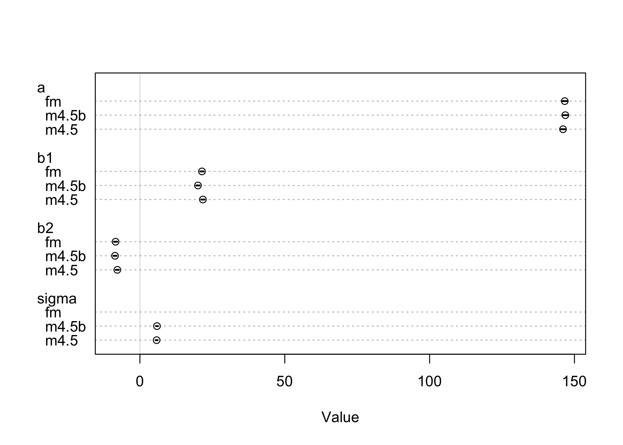
How different are the models?
Question 4
For this problem, we’re going to reuse the same model (m4.5) from Question 3 and run prior predictive simulations to understand the role of different priors. For help, see 5.4-5.5 code in the book.
m4.5 <- quap(
  alist(
    height ~ dnorm( mu , sigma ) ,
    mu <- a + b1*(weight_s) + b2 * weight_s2,
    a ~ dnorm( 178 , 20 ) ,
    b1 ~ dlnorm( 0 , 1 ) ,
    b2 ~ dnorm( 0, 1 ) ,
    sigma ~ dunif( 0 , 50 )
) , data=d )
set.seed(45)
prior <- extract.prior(m4.5)
precis(prior)
##               mean         sd        5.5%      94.5%     histogram
## a     177.60867247 20.7249835 144.1785056 211.421234      ▁▁▃▇▇▂▁▁
## b1      1.61236478  1.8754510   0.1867143   4.433442    ▇▂▁▁▁▁▁▁▁▁
## b2     -0.05036862  0.9688063  -1.6422983   1.447121 ▁▁▁▂▃▅▇▇▅▃▁▁▁
## sigma  25.14432248 14.5856372   2.5161320  47.371388    ▇▇▅▇▇▇▇▇▇▇
w_seq <- seq( from=min(d$weight_s) , to=max(d$weight_s) , length.out=50 )
w2_seq <- w_seq^2
mu <- link( m4.5 , post=prior , data=list( weight_s=w_seq , weight_s2=w2_seq ) )
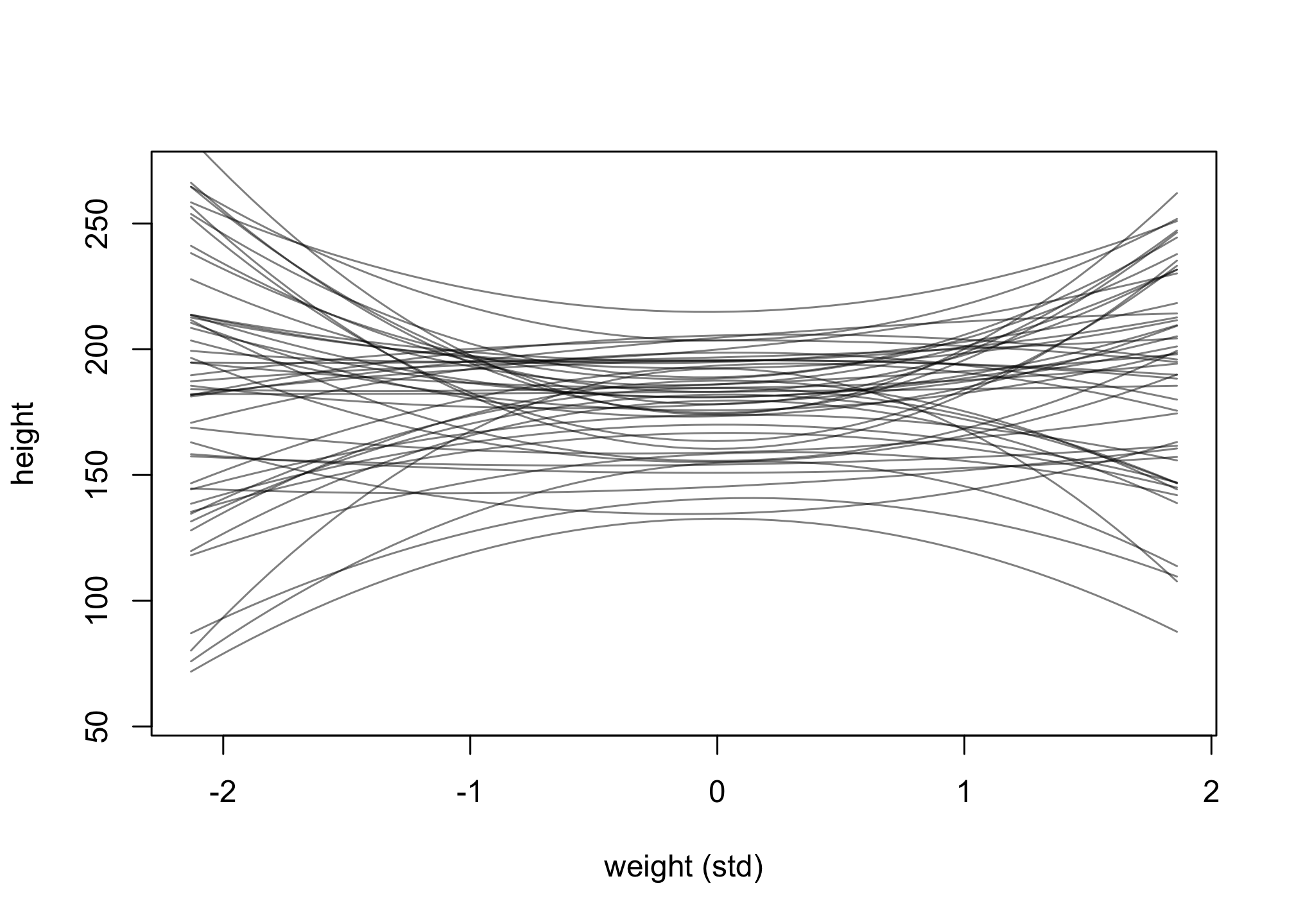
plot( NULL , xlim=range(w_seq) , ylim=c(55,270) ,
xlab="weight (std)" , ylab="height" )
for ( i in 1:50 ) lines( w_seq , mu[i,] , col=col.alpha("black",0.5) )
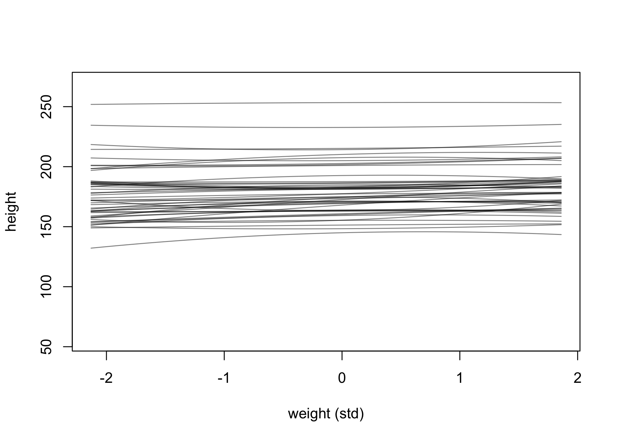
Change the priors on the b2 coefficient to b2 ~ dnorm(0, 10) and rerun the prior predictive simulation.
m4.5_alter <- quap(
alist(
height ~ dnorm( mu , sigma ) ,
mu <- a + b1*(weight_s) + b2 * weight_s2,
a ~ dnorm( 178 , 20 ) ,
b1 ~ dlnorm(0, 1) ,
b2 ~ dnorm(0, 10) , # updated prior
sigma ~ dunif( 0 , 50 )
) , data=d )
prior <- extract.prior(m4.5_alter)
mu <- link( m4.5_alter , post=prior , data=list( weight_s=w_seq , weight_s2=w2_seq ) )
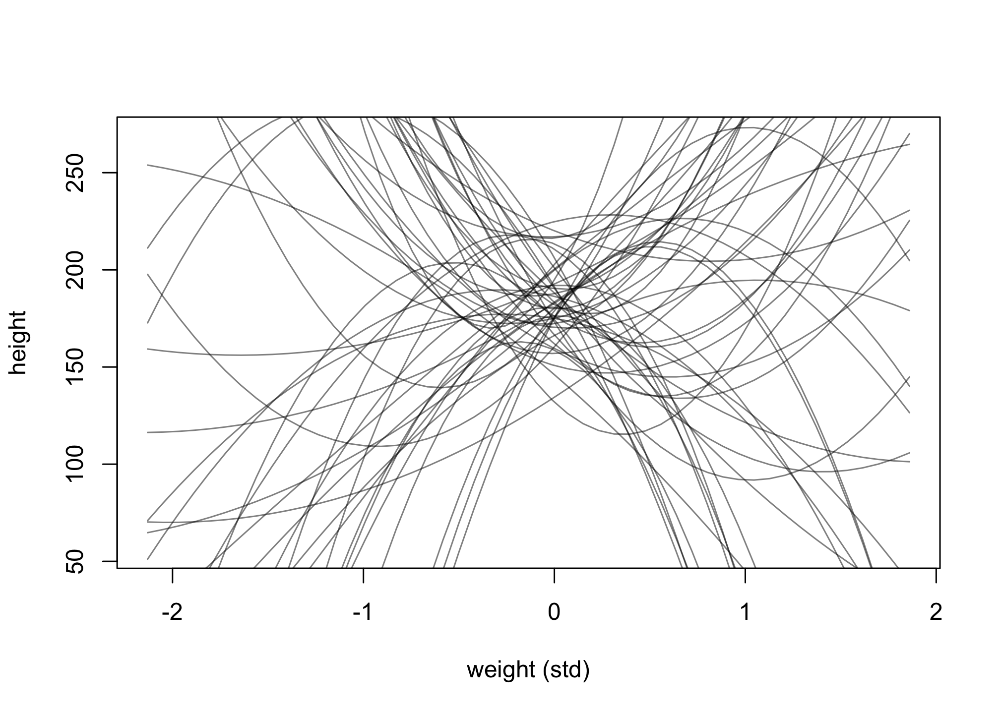
plot( NULL , xlim=range(w_seq) , ylim=c(55,270) ,
xlab="weight (std)" , ylab="height" )
for ( i in 1:50 ) lines( w_seq , mu[i,] , col=col.alpha("black",0.5) )
Now, change the priors on the beta coefficients to more “flat, very uninformative” priors, dnorm(0, 100) for b1 and b2. Rerun a similar prior predictive simulation.
m4.5_flat <- quap(
  alist(
    height ~ dnorm( mu , sigma ) ,
    mu <- a + b1*(weight_s) + b2 * weight_s2,
    a ~ dnorm( 178 , 20 ) ,
    b1 ~ dnorm(0, 100) , # very flat priors
    b2 ~ dnorm(0, 100) , # very flat priors
    sigma ~ dunif( 0 , 50 )
) , data=d )

prior <- extract.prior(m4.5_flat)

mu <- link( m4.5_flat , post=prior , data=list( weight_s=w_seq , weight_s2=w2_seq ) )

plot( NULL , xlim=range(w_seq) , ylim=c(55,270) ,
xlab="weight (std)" , ylab="height" )
for ( i in 1:50 ) lines( w_seq , mu[i,] , col=col.alpha("black",0.5) )
What are the consequences for using a flatter prior? Explain what you suspect is occuring.
Optional Challenge (Not graded)
Return to data(cherry_blossoms) and model the association between blossom date (day) and March temperature (temp). Note that there are many missing values in both variables. You may consider a linear model, a polynomial, or a spline on temperature. How well does temperature trend predict the blossom trend?
First, let’s look for missing values.
library(rethinking)
data(cherry_blossoms)
colSums( is.na(cherry_blossoms) )
##       year        doy       temp temp_upper temp_lower
##          0        388         91         91         91
Let’s just select doy and temp.
d <- cherry_blossoms
d2 <- d[ complete.cases( d$doy , d$temp ) , c("doy","temp") ]
# other ways to write this using tidyverse
# d2 <- tidyr::drop_na(d, c("doy","temp"))
# d2 <- dplyr::filter(d, !is.na("doy") | !is.na("temp"))
num_knots <- 30
knot_list <- quantile( d2$temp , probs=seq(0,1,length.out=num_knots) )
library(splines)
B <- bs(d2$temp,
knots=knot_list[-c(1,num_knots)] ,
degree=3 , intercept=TRUE )
m4H5 <- quap(
  alist(
    D ~ dnorm( mu , sigma ) ,
    mu <- a + B %*% w ,
    a ~ dnorm(100,10),
    w ~ dnorm(0,10),
    sigma ~ dexp(1)
    ),
  data=list( D=d2$doy , B=B ) ,
  start=list( w=rep( 0 , ncol(B) ) )
  )
You can inspect the precis output, if you like. The weights aren’t going to be meaningful to you. Let’s plot. The only trick here is to get the order of the temperature values right when we plot, since they are not ordered in the data or in the basis functions. We can do this with order to get the index values for the proper order and then index everything else by this:
mu <- link( m4H5 )
mu_mean <- apply( mu , 2 , mean )
mu_PI <- apply( mu , 2 , PI, 0.97 )
plot( d2$temp , d2$doy , col=col.alpha(rangi2,0.3) , pch=16 ,
xlab="temp" , ylab="doy" )
o <- order( d2$temp )
lines( d2$temp[o] , mu_mean[o] , lwd=3 )
shade( mu_PI[,o] , d2$temp[o] , col=grau(0.3) )
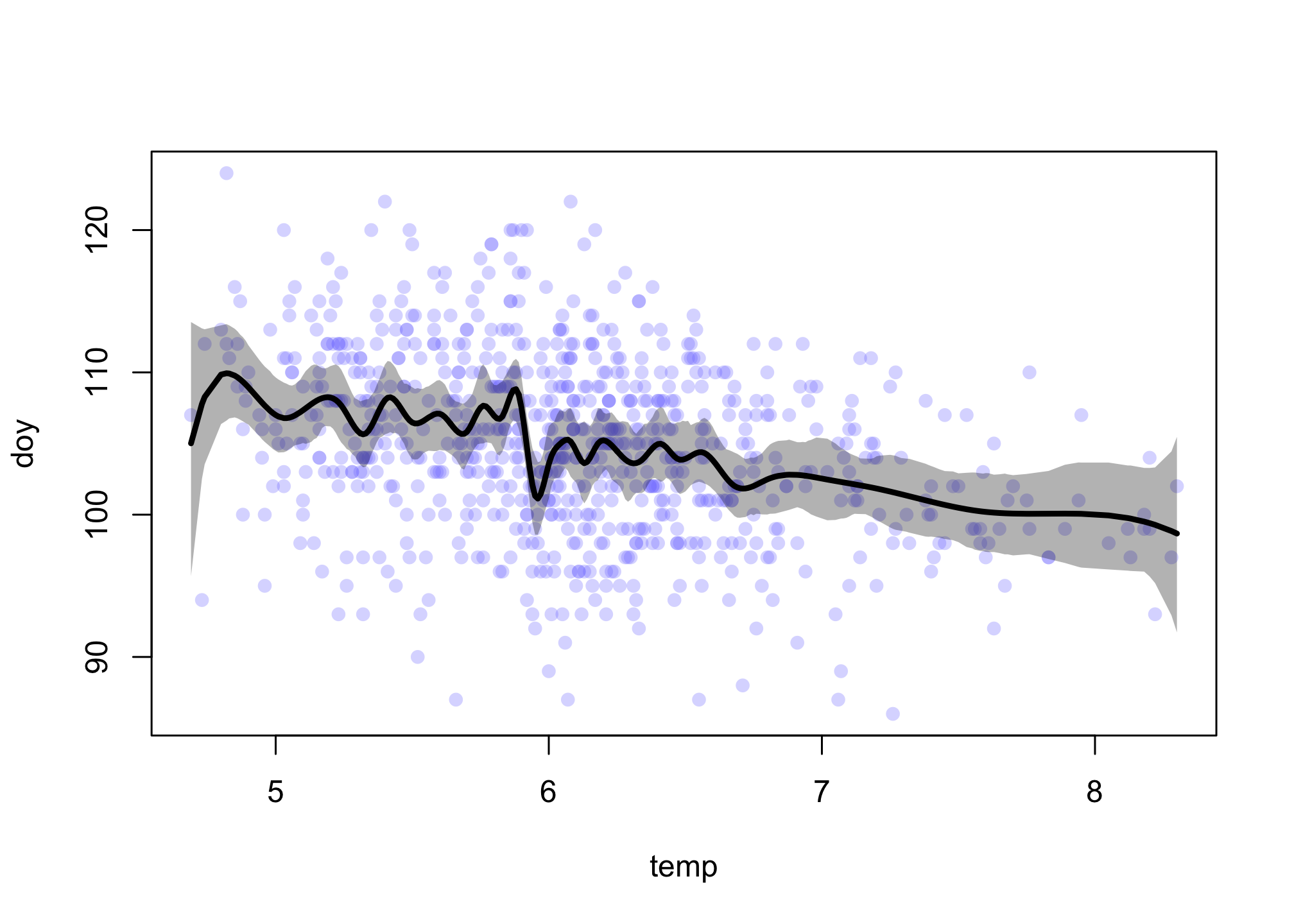
There is a silly amount of wiggle in this spline. I used 30 knots and quite loose prior weights, so this wiggle isn’t unexpected. It also probably isn’t telling us anything causal. Overall the trend is quite linear, aside from the odd drop just before 6 degrees. This could be real, or it could be an artifact of changes in the record keeping. The colder dates are also older and the temperatures for older dates were estimated differently.