Problem Set 3

This problem set is due on February 21, 2022 at 11:59am.

Step 1: Download this file locally.

Step 2: Complete the assignment

Step 3: Knit the assignment as either an html or pdf file.

Step 4: Submit your file here through this canvas link.

• Name:
• UNCC ID:
• Other student worked with (optional):

Question 1

From the Howell1 dataset, consider only the people younger than 13 years old. Estimate the causal association between age and weight. Assume that age influences weight through two paths. First, age influences height, and height influences weight. Second, age directly influences weight through age related changes in muscle growth and body proportions. All of this implies this causal model (DAG):

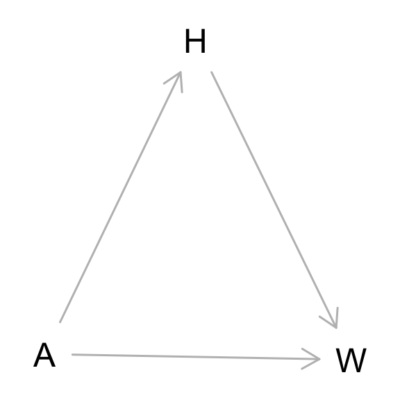
Use a linear regression to estimate the total (not just direct) causal effect of each year of growth on weight. Be sure to carefully consider the priors. Try using prior predictive simulation to assess what they imply.

Question 2

Now suppose the causal association between age and weight might be different for boys and girls. Use a single linear regression, with a categorical variable for sex, to estimate the total causal effect of age on weight separately for boys and girls. How do girls and boys differ? Provide one or more posterior contrasts as a summary.

Question 3

For this problem, we want to compare the difference between Frequentist and Bayesian linear regressions. We’re going to use the similar functions from section 4.5.

To begin, I have provided the same code to get the model m4.5 (i.e., run R code 4.65). Please run it and refresh yourself.

# R code 4.65 + 4.66 (precis)
library(rethinking)
data(Howell1)
d <- Howell1
d$weight_s <- ( d$weight - mean(d$weight) )/sd(d$weight)
d$weight_s2 <- d$weight_s^2

m4.5 <- quap(
  alist(
    height ~ dnorm( mu , sigma ) ,
    mu <- a + b1*(weight_s) + b2 * weight_s2,
    a ~ dnorm( 178 , 20 ) ,
    b1 ~ dlnorm( 0 , 1 ) ,
    b2 ~ dnorm( 0, 1 ) ,
    sigma ~ dunif( 0 , 50 )
) , data=d )

precis( m4.5 )

##             mean        sd       5.5%      94.5%
## a     146.058157 0.3689835 145.468450 146.647864
## b1     21.732164 0.2888954  21.270453  22.193874
## b2     -7.802966 0.2741948  -8.241182  -7.364750
## sigma   5.774674 0.1764807   5.492623   6.056724

Now modify m4.5 model by relaxing our “positive relationship” (aka lognormal) assumption for the b1 variable by modifying it’s prior as dnorm( 0 , 1 ) and create a new model called m4.5b. Run precis(m4.5b).

Now, run a frequentist regression of m4.5b by using the lm function. I have provided this code.

# hint: you need to only remove the eval=FALSE so this code runs
fm <- lm(height ~ weight_s + weight_s2, data = d)
names(fm$coefficients) <- c('a','b1','b2') # rename coef for consistency
fm

Now compare all three models by using the coeftab() and putting all three of the models as parameters. You can also run a plot() on the coeftab() function to run a plot of the effects.

How different are the models?

Question 4

For this problem, we’re going to reuse the same model (m4.5) from Question 3 and run prior predictive simulations to understand the role of different priors. For help, see 5.4-5.5 code in the book.

Change the priors on the b2 coefficient to b2 ~ dnorm(0, 10) and rerun the prior predictive simulation.

Now, change the priors on the beta coefficients to more “flat, very uninformative” priors, dnorm(0, 100) for b1 and b2. Rerun a similar prior predictive simulation.

What is the impact of using more flat/uninformative priors? Which of the three priors do you think is most reasonable to use?

Optional Challenge (Not graded)

Return to data(cherry_blossoms) and model the association between blossom date (day) and March temperature (temp). Note that there are many missing values in both variables. You may consider a linear model, a polynomial, or a spline on temperature. How well does temperature trend predict the blossom trend?