Problem Set 2 Solutions
This problem set is due on February 6, 2022 at 11:59am.
Question 1
Construct a linear regression of weight as predicted by height, using the adults (age 18 or greater) from the Howell1 dataset. The heights listed below were recorded in the !Kung census, but weights were not recorded for these individuals.
Provide predicted weights and 89% compatibility intervals for each of these individuals. Fill in the table below, using model-based predictions.
library(rethinking)
data(Howell1)
d <- Howell1[Howell1$age>=18,]

dat <- list(W = d$weight, H = d$height, Hbar = mean(d$height))

m_adults <- quap(
    alist(
        W ~ dnorm( mu , sigma ) ,
        mu <- a + b*( H - Hbar ),
        a ~ dnorm( 60 , 10 ) ,
        b ~ dlnorm( 0 , 1 ) ,
        sigma ~ dunif( 0 , 10 )
    ) , data=dat )

set.seed(100)
sample_heights = c(140,150,160,175)

simul_weights <- sim( m_adults , data=list(H=sample_heights,Hbar=mean(d$height)))

# simulated means
mean_weights = apply( simul_weights , 2 , mean )
# simulated PI's
pi_weights = apply( simul_weights , 2 , PI , prob=0.89 )

df <- data.frame(
  individual = 1:4,
  sample_heights = sample_heights,
  simulated_mean = mean_weights,
  low_pi = pi_weights[1,],
  high_pi = pi_weights[2,]
)

df
##   individual sample_heights simulated_mean   low_pi  high_pi
## 1          1            140       35.66492 28.94471 42.53722
## 2          2            150       42.15074 35.55812 48.65086
## 3          3            160       48.56264 41.84482 55.16735
## 4          4            175       57.88451 51.56018 64.33351
col_name <- c('Individual','Height', 'Expected Weight', 'Low Interval', 'High Interval')
# see https://bookdown.org/yihui/rmarkdown-cookbook/kable.html
# fyi this is a way to "fancy" print dataframe in RMarkdown
knitr::kable(df, col.names = col_name)
| Individual | Height | Expected Weight | Low Interval | High Interval |
|---|---|---|---|---|
| 1 | 140 | 35.66492 | 28.94471 | 42.53722 |
| 2 | 150 | 42.15074 | 35.55812 | 48.65086 |
| 3 | 160 | 48.56264 | 41.84482 | 55.16735 |
| 4 | 175 | 57.88451 | 51.56018 | 64.33351 |
Questions 2-4
A sample of students is measured for height each year for 3 years. After the third year, you want to fit a linear regression predicting height (in centimeters) using year as a predictor.
Question 2:
- Write down a mathematical model definition for this regression, using any variable names and priors you choose. You don’t need to run since you won’t have the data. You may also write down your equation and then upload an image.
We’ll define as the outcome variable height \(h_{ij}\), where
\(h_{ij} \sim Normal(u_{ij},\sigma)\)
\(\mu_{ij} = \alpha + \beta * (x_{j} - \bar{x})\)
\(\alpha \sim Normal(100, 10)\)
\(\beta \sim Normal(0, 10)\)
\(\sigma \sim Exponential(1)\)
where h is height and y is year and y the average year in the sample. The index i indicates the student and the index j indicates the year
The problem didn’t say how old the students are, so you’ll have to decide for yourself. The priors above assume the students are still growing, so the mean height α is set around 100 cm. The slope with year β is vague here—we’ll do better in the next problem. For σ, this needs to express how variable students are in the same year
Question 3
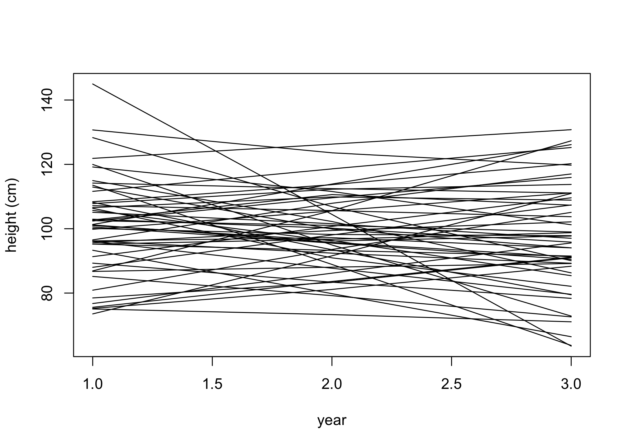
- Run prior predictive simulation and defend your choice of priors.
n <- 50
a <- rnorm( n , 100 , 10 )
b <- rnorm( n , 0 , 10 )
s <- rexp( n , 1 )

x <- 1:3
xbar <- mean(x)
# matrix of heights, students in rows and years in columns
h <- matrix( NA , nrow=n , ncol=3 )
for ( i in 1:n ) for ( j in 1:3 )
  h[ i , j ] <- rnorm( 1 , a[i] + b[i]*( x[j] - xbar ) , s[i] )

plot( NULL , xlim=c(1,3) , ylim=range(h) , xlab="year" , ylab="height (cm)" )
for ( i in 1:n ) lines( 1:3 , h[i,] )
Question 4
Now suppose I tell you that the students were 8 to 10 years old (so 8 year 1, 9 year 2, etc.). What do you expect of the trend of students’ heights over time?
- Does this information lead you to change your choice of priors? How? Resimulate your priors from Question 3.
A simple way to force individuals to get taller from one year to the next is to constrain the slope β to be positive. A log-normal distribution makes this rather easy, but you do have to be careful in choosing its parameter values. Recall that the mean of a log-normal is \(exp(\mu + \sigma^{2} / 2)\). Let’s try \(\mu = 1\) and \(\sigma = 0.5\). This will give a mean \(exp(1 + (0.25)^{2} / 2) ≈ 3\), or 3 cm of growth per year.
n <- 50
a <- rnorm( n , 100 , 10 )
b <- rlnorm( n , 1 , 0.5 )
s <- rexp( n , 1 )
x <- 1:3
xbar <- mean(x)
# matrix of heights, students in rows and years in columns
h <- matrix( NA , nrow=n , ncol=3 )
for ( i in 1:n ) for ( j in 1:3 )
  h[ i , j ] <- rnorm( 1 , a[i] + b[i]*( x[j] - xbar ) , s[i] )
plot( NULL , xlim=c(1,3) , ylim=range(h) , xlab="year" , ylab="height (cm)" )
  for ( i in 1:n ) lines( 1:3 , h[i,] )
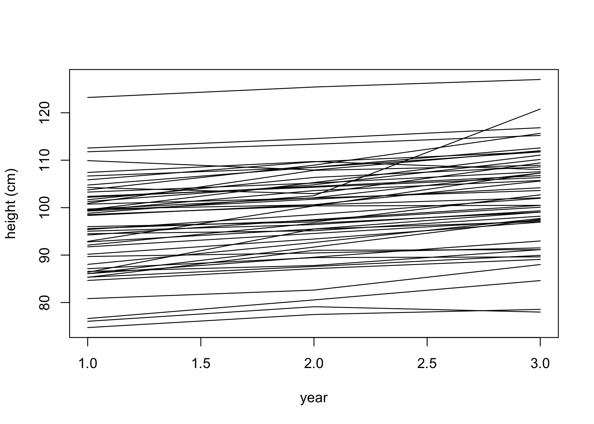
Aside from a few people, the lines are slope upwards. Why do some of them zig-zag? Because the variation around the expectation from σ allows it. If you think of this as measurement error, it’s not necessarily bad. If measurement error is small however, you’d have to think harder. Much later in the book, you’ll learn some tools to help with this kind of problem.
Question 5
4. Refit model m4.3 from the chapter, but omit the mean weight xbar this time. Compare the new model’s posterior to that of the original model. In particular, look at the covariance among the parameters. What is different? Then compare the posterior predictions of both models.
library(rethinking)
data(Howell1);
d <- Howell1;
d2 <- d[ d$age >= 18 , ]

xbar <- mean(d2$weight)
# run original model from code
m4.3 <- quap(
  alist(
    height ~ dnorm( mu , sigma ) ,
    mu <- a + b*(weight - xbar),
    a ~ dnorm( 178 , 20 ) ,
    b ~ dlnorm( 0 , 1 ) ,
    sigma ~ dunif( 0 , 50 )
) , data=d2 )
precis( m4.3 )
##              mean         sd        5.5%       94.5%
## a     154.6012818 0.27029702 154.1692950 155.0332687
## b       0.9032859 0.04192198   0.8362865   0.9702853
## sigma   5.0716813 0.19113598   4.7662091   5.3771535
m4.3b <- quap(
  alist(
    height ~ dnorm( mu , sigma ) ,
    mu <- a + b*weight ,
    a ~ dnorm( 178 , 20 ) ,
    b ~ dlnorm( 0 , 1 ) ,
    sigma ~ dunif( 0 , 50 )
) , data=d2 )
precis( m4.3b )
##            mean         sd        5.5%       94.5%
## a     114.53431 1.89774691 111.5013449 117.5672771
## b       0.89073 0.04175798   0.8239927   0.9574674
## sigma   5.07272 0.19124901   4.7670668   5.3783725
Notice that the models yield similar outputs except for the a coefficients.
Let’s now look at the covariation which is due to running quadratic approximation.
round( vcov( m4.3 ) , 2 )
##          a b sigma
## a     0.07 0  0.00
## b     0.00 0  0.00
## sigma 0.00 0  0.04
Focus on the off-diagonals … we see nearly zero covariation. This is good.
We can also view this through the pairs() function.
pairs(m4.3)
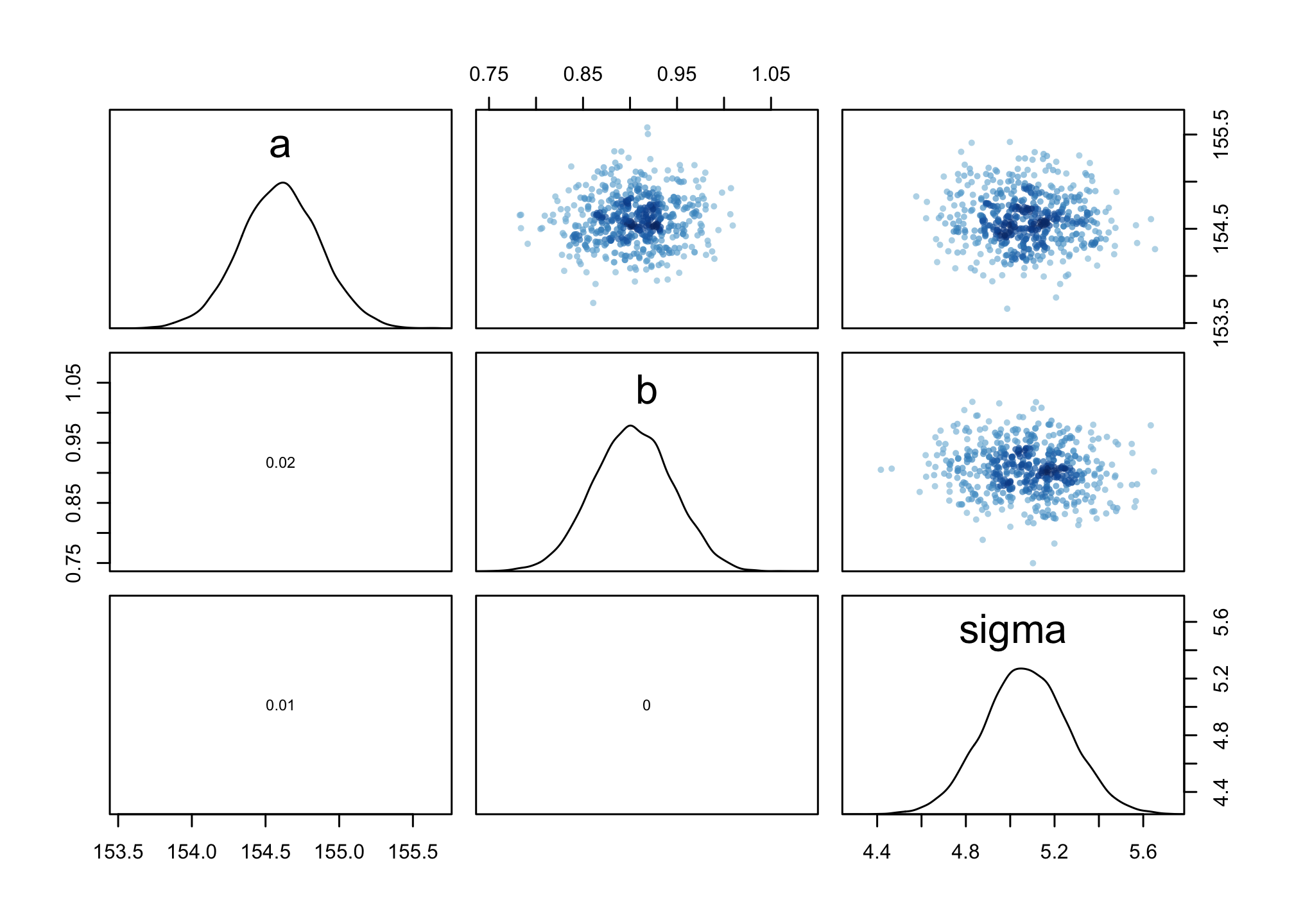
Look at the cov(A,B) plot. Notice there’s no covariation.
While if we do this for the non-scaled, we’ll see something different. First, let’s just run covariation.
round( vcov( m4.3b ) , 2 )
##           a     b sigma
## a      3.60 -0.08  0.01
## b     -0.08  0.00  0.00
## sigma  0.01  0.00  0.04
Notice some covariation (-0.08) for the non-scaled. While -0.08 covariation isn’t much, let’s translate this into correlation (as covariation depends on the scale of variables).
round( cov2cor(vcov( m4.3b )) , 2 )
##           a     b sigma
## a      1.00 -0.99  0.03
## b     -0.99  1.00 -0.03
## sigma  0.03 -0.03  1.00
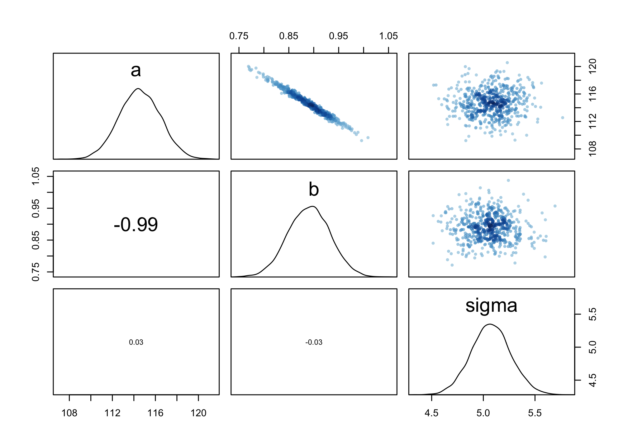
Wow – unscaled our A-B are nearly -1 negative correlation. We’ll see this in the pairs() function.
pairs(m4.3b)
We can also run posterior prediction simulations.
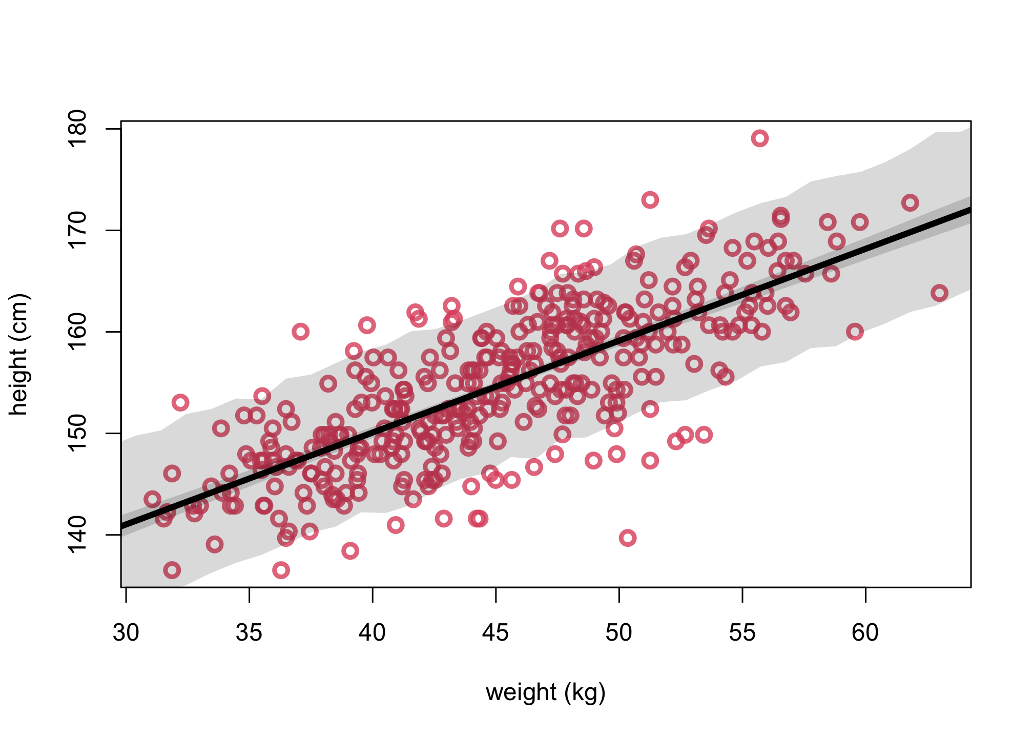
First, let’s run the original model (scaled).
col2 <- col.alpha(2,0.8)
# get posterior mean via link function
xseq <- seq(from=0,to=75,len=75)
mean = mean(d2$weight)
mu <- link(m4.3,data=list(weight = xseq, xbar = mean))
mu.mean <- apply( mu , 2 , mean )
mu.PI <- apply( mu , 2 , PI , prob=.89)
# get posterior predictions via sim function
sim.weight <- sim( m4.3 , data=list(weight = xseq, Wbar = mean(d2$weight)))
weight.PI <- apply( sim.weight , 2 , PI , prob=0.89 )

plot(d2$weight, d2$height, col=col2, lwd=3,
     cex=1.2, xlab="weight (kg)", ylab="height (cm)")
lines(xseq, mu.mean, lwd=4)
shade( mu.PI , xseq )
shade( weight.PI , xseq )
Now run the unscaled model simulations.
col2 <- col.alpha(2,0.8)
# get posterior mean via link function
xseq <- seq(from=0,to=75,len=75)
mean = mean(d2$weight)
mu <- link(m4.3b,data=list(weight = xseq))
mu.mean <- apply( mu , 2 , mean )
mu.PI <- apply( mu , 2 , PI , prob=.89)
# get posterior predictions via sim function
sim.weight <- sim( m4.3b , data=list(weight = xseq, Wbar = mean(d2$weight)))
weight.PI <- apply( sim.weight , 2 , PI , prob=0.89 )

plot(d2$weight, d2$height, col=col2, lwd=3,
     cex=1.2, xlab="weight (kg)", ylab="height (cm)")
lines(xseq, mu.mean, lwd=4)
shade( mu.PI , xseq )
shade( weight.PI , xseq )
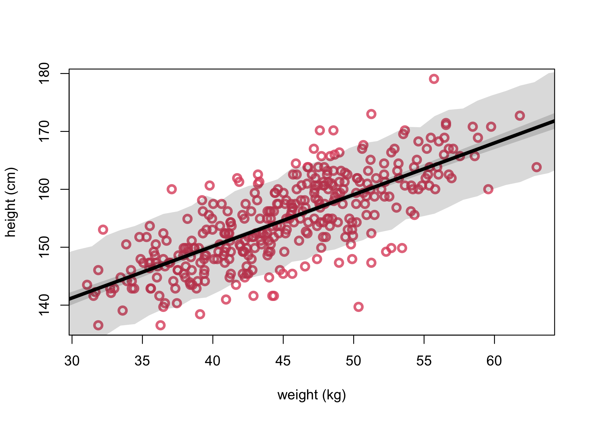
We have the conclusion that while these models make the same posterior predictions, but the parameters have quite different meanings and relationships with one another. There is nothing wrong with this new version of the model. But usually it is much easier to set priors, when we center the predictor variables. But you can always use prior simulations to set sensible priors, when in doubt.
Package versions
sessionInfo()
## R version 4.1.1 (2021-08-10)
## Platform: aarch64-apple-darwin20 (64-bit)
## Running under: macOS Monterey 12.1
##
## Matrix products: default
## BLAS:   /Library/Frameworks/R.framework/Versions/4.1-arm64/Resources/lib/libRblas.0.dylib
## LAPACK: /Library/Frameworks/R.framework/Versions/4.1-arm64/Resources/lib/libRlapack.dylib
##
## locale:
## [1] en_US.UTF-8/en_US.UTF-8/en_US.UTF-8/C/en_US.UTF-8/en_US.UTF-8
##
## attached base packages:
## [1] parallel  stats     graphics  grDevices datasets  utils     methods
## [8] base
##
## other attached packages:
## [1] rethinking_2.21      cmdstanr_0.4.0.9001  rstan_2.21.3
## [4] ggplot2_3.3.5        StanHeaders_2.21.0-7
##
## loaded via a namespace (and not attached):
##  [1] sass_0.4.0           jsonlite_1.7.2       bslib_0.3.1
##  [4] RcppParallel_5.1.4   assertthat_0.2.1     posterior_1.1.0
##  [7] distributional_0.2.2 highr_0.9            stats4_4.1.1
## [10] tensorA_0.36.2       renv_0.14.0          yaml_2.2.1
## [13] pillar_1.6.4         backports_1.4.1      lattice_0.20-44
## [16] glue_1.6.0           uuid_1.0-3           digest_0.6.29
## [19] checkmate_2.0.0      colorspace_2.0-2     htmltools_0.5.2
## [22] pkgconfig_2.0.3      bookdown_0.24        purrr_0.3.4
## [25] mvtnorm_1.1-3        scales_1.1.1         processx_3.5.2
## [28] tibble_3.1.6         generics_0.1.1       farver_2.1.0
## [31] ellipsis_0.3.2       withr_2.4.3          cli_3.1.0
## [34] mime_0.12            magrittr_2.0.1       crayon_1.4.2
## [37] evaluate_0.14        ps_1.6.0             fs_1.5.0
## [40] fansi_0.5.0          MASS_7.3-54          pkgbuild_1.3.1
## [43] blogdown_1.5         tools_4.1.1          loo_2.4.1
## [46] prettyunits_1.1.1    lifecycle_1.0.1      matrixStats_0.61.0
## [49] stringr_1.4.0        munsell_0.5.0        callr_3.7.0
## [52] compiler_4.1.1       jquerylib_0.1.4      rlang_0.4.12
## [55] grid_4.1.1           rstudioapi_0.13      base64enc_0.1-3
## [58] rmarkdown_2.11       xaringanExtra_0.5.5  gtable_0.3.0
## [61] codetools_0.2-18     inline_0.3.19        abind_1.4-5
## [64] DBI_1.1.1            R6_2.5.1             gridExtra_2.3
## [67] lubridate_1.8.0      knitr_1.36           dplyr_1.0.7
## [70] fastmap_1.1.0        utf8_1.2.2           downloadthis_0.2.1
## [73] bsplus_0.1.3         KernSmooth_2.23-20   shape_1.4.6
## [76] stringi_1.7.6        Rcpp_1.0.7           vctrs_0.3.8
## [79] tidyselect_1.1.1     xfun_0.28            coda_0.19-4