Problem Set 1 Solutions
This problem set is due on January 31, 2022 at 11:59am.
Question 1
Your friend just became interested in Bayesian statistics. In one paragraph or less (no code), explain the following to them: * Why/when is Bayesian statistics useful?
Many answers are sufficient.
Bayesian statistics are useful in situations where (see Kay et al. CHI 2016):
- Bayesian analysis provides more precise estimates of previously-studied conditions in each successive study.
- Bayesian analysis allows more precise comparison of novel conditions against known conditions.
- Bayesian analysis draws more reasonable conclusions from small-n studies.
- Bayesian analyses help shift the conversation from “Does it work?” to “How strong is the effect?” “How confident are we in this estimate?” and “Should we care?”
- What are the similarities in Bayesian and frequentist statistics?
Bayesian and frequentist analyses share a common goal: to learn from data about the world around us. They differ in how they interpret probabilities. Bayesians interpret probabilities as a “degree of belief” while Frequentists interpret probabilities as a “long run relative frequency.”
In essence, Frequentist statistics can be thought of as a subset of Bayesian statistics in which we have no prior information or when our sample size is so large, that our prior no longer has any weight in our posterior. In those cases, typically Frequentist and Bayesian statistics produce very similar results.
Question 2
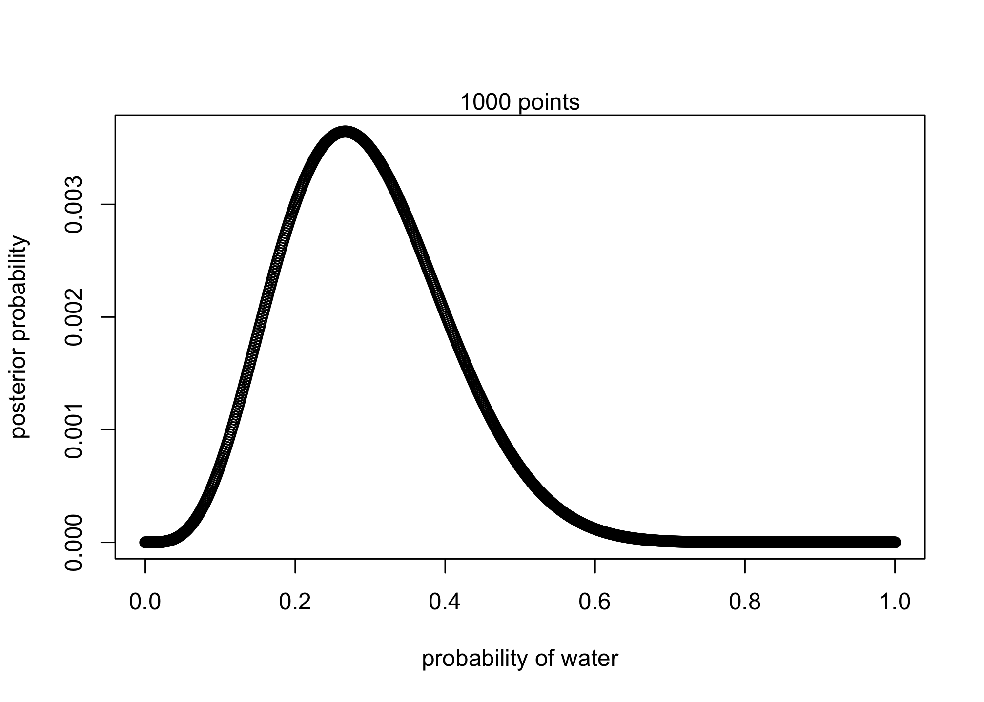
Suppose the globe tossing data (Chapter 2) had turned out to be 4 water and 11 land. Construct the posterior distribution, using grid approximation. Use the same flat prior as in the book.
## R code 2.3
set.seed(100)
# define grid
p_grid <- seq( from=0 , to=1 , length.out=1000 )

# define prior
prior <- rep( 1 , 1000 )

# compute likelihood at each value in grid
likelihood <- dbinom( 4 , size=15 , prob=p_grid )

# compute product of likelihood and prior
unstd.posterior <- likelihood * prior

# standardize the posterior, so it sums to 1
posterior <- unstd.posterior / sum(unstd.posterior)

plot( p_grid , posterior , type="b" ,
    xlab="probability of water" , ylab="posterior probability" )
mtext( "1000 points" )
Question 3
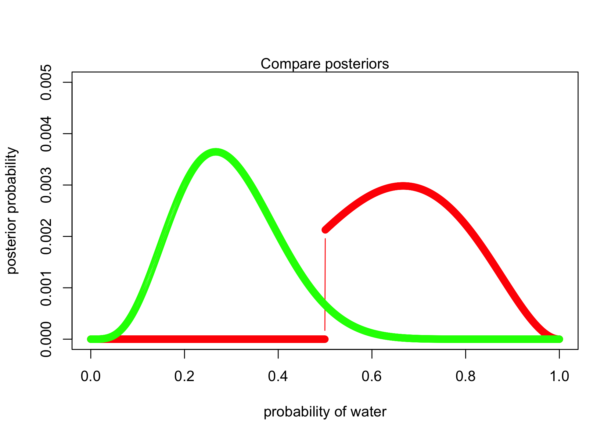
Now suppose the data are 4 water and 2 land. Compute the posterior again, but this time use a prior that is zero below p = 0.5 and a constant above p = 0.5. This corresponds to prior information that a majority of the Earth’s surface is water. Compare the new posterior with the previous posterior (flat)
## R code 2.3
# define grid
p_grid <- seq( from=0 , to=1 , length.out=1000 )
# define prior
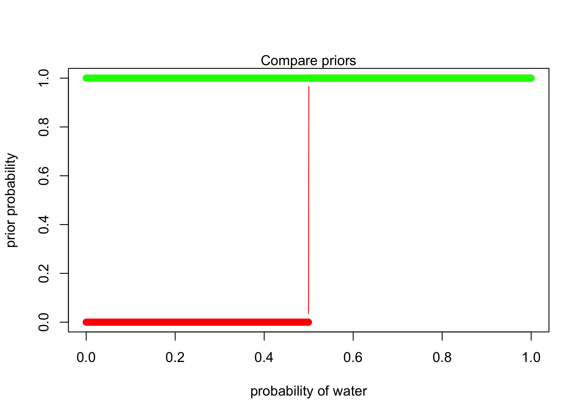
post_prior <- ifelse( p_grid < 0.5 , 0 , 1 )
# compute likelihood at each value in grid
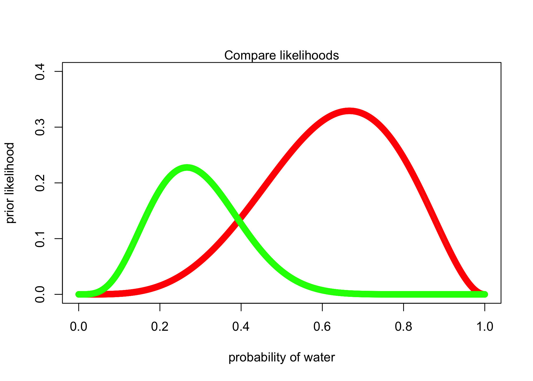
post_likelihood <- dbinom( 4 , size=6 , prob=p_grid )
# compute product of likelihood and prior
post_unstd.posterior <- post_likelihood * post_prior
# standardize the posterior, so it sums to 1
post_posterior <- post_unstd.posterior / sum(post_unstd.posterior)
plot( p_grid , post_posterior , type="b" , col = "red",
xlab="probability of water" , ylab="posterior probability", ylim=c(0, 0.005) )
lines(p_grid , posterior , type="b" , col = "green")
mtext( "Compare posteriors" )
plot( p_grid , post_prior , type="b" , col = "red",
    xlab="probability of water" , ylab="prior probability", ylim=c(0, 1) )
lines(p_grid , prior , type="b" , col = "green")
mtext( "Compare priors" )
plot( p_grid , post_likelihood , type="b" , col = "red",
    xlab="probability of water" , ylab="prior likelihood", ylim=c(0, .4) )
lines(p_grid , likelihood , type="b" , col = "green")
mtext( "Compare likelihoods" )
Question 4
For the posterior distribution from 3, compute 89% percentile and HPDI intervals. Compare the widths of these intervals. Which is wider? Why? If you had only the information in the interval, what might you misunderstand about the shape of the posterior distribution?
library(rethinking)
#calculate samples of post_posterior
samples <- sample(p_grid, size = 1e4, replace = TRUE, prob=post_posterior)

# 89 percentile
PI(samples, prob=.89)
##        5%       94%
## 0.5245245 0.8798799
# HPDI
HPDI(samples, prob=.89)
##     |0.89     0.89|
## 0.5005005 0.8388388
HPDI is densest (narrowest) region with 89% mass, thus PI is wider than HPDI.
With only intervals, an analyst would miss the drop in the posterior’s shape below 52% due to the prior that assumes greater than 50%.
Optional Question (Not graded)
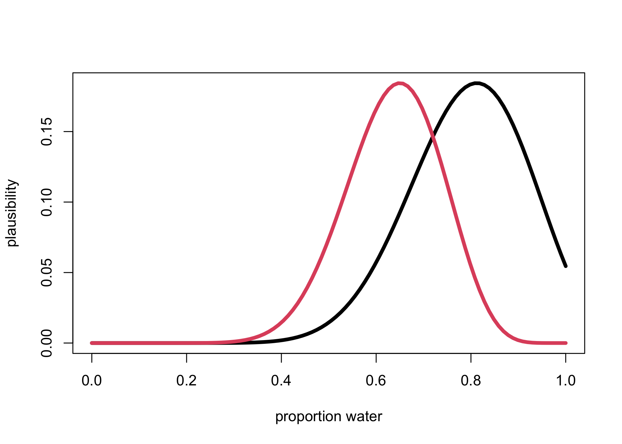
Suppose there is bias in sampling so that Land is more likely than Water to be recorded. Specifically, assume that 1-in-5 (20%) of Water samples are accidentally recorded instead as “Land.” First, write a generative simulation of this sampling process. Assuming the true proportion of Water is 0.70, what proportion does your simulation tend to produce instead?
# Pr(W|W) = 0.8
# Pr(W|L) = 0.2
# Pr(W) = 0.7*0.8
set.seed(100)
true_prob = 0.7
bias = 0.2
N=10000

# assume 1 = water, 0 = land
trueW <- rbinom(N,size=20,prob=true_prob)
obsW <- rbinom(N,size=trueW,prob=1-bias)
mean(obsW/20)
## [1] 0.560355
# or
W <- rbinom(N,size=20,prob=true_prob*(1-bias))

mean(W/20)
## [1] 0.560975
Second, using a simulated sample of 20 tosses, compute the unbiased posterior distribution of the true proportion of water.
# now analyze
# Pr(p|W,N) = Pr(W|p,N)Pr(p) / Z
# Pr(W|N,p) = Pr(W)Pr(W|W)

W <- rbinom(1,size=20,prob=0.7*0.8)
# grid approx
grid_p <- seq(from=0,to=1,len=100)
pr_p <- dbeta(grid_p,1,1)
prW <- dbinom(W,20,grid_p*0.8)
post <- prW*pr_p

post_bad <- dbinom(W,20,grid_p)

plot(grid_p,post,type="l",lwd=4,xlab="proportion water",ylab="plausibility")
lines(grid_p,post_bad,col=2,lwd=4)
tidyverse
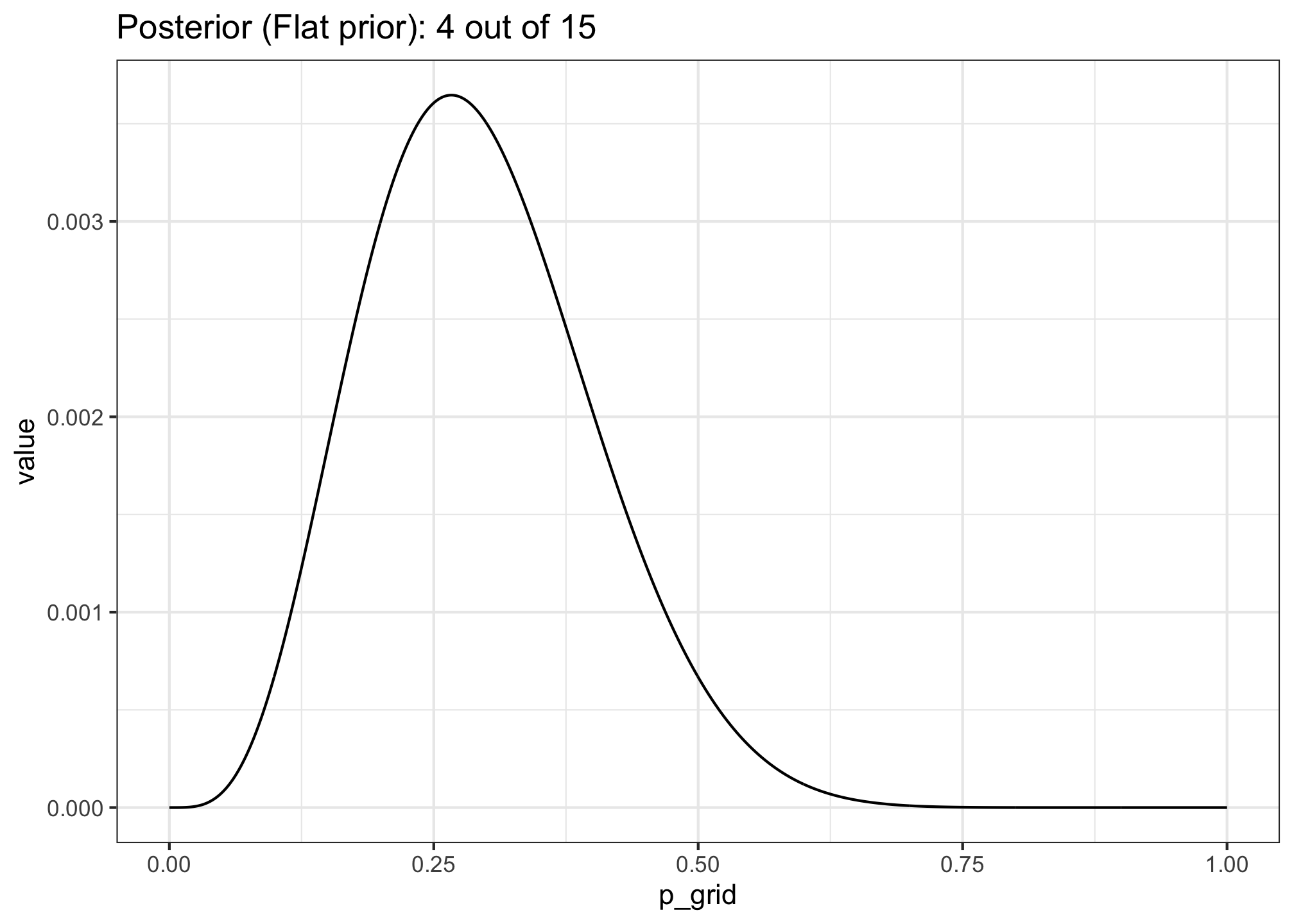
- Suppose the globe tossing data (Chapter 2) had turned out to be 4 water and 11 land. Construct the posterior distribution, using grid approximation. Use the same flat prior as in the book.
# tidyverse approach
library(tidyverse)
# how many grid points would you like?
n <- 1000
n_success <- 4
n_trials  <- 15

d <-
  tibble(p_grid = seq(from = 0, to = 1, length.out = n),
         # note we're still using a flat uniform prior
         prior  = 1) %>%
  mutate(likelihood = dbinom(n_success, size = n_trials, prob = p_grid)) %>%
  mutate(posterior = (likelihood * prior) / sum(likelihood * prior))

d %>%
  pivot_longer(-p_grid) %>%
  filter(name == "posterior") %>%
  ggplot(aes(x = p_grid, y = value)) +
  geom_line() +
  ggtitle("Posterior (Flat prior): 4 out of 15") +
  theme_bw()
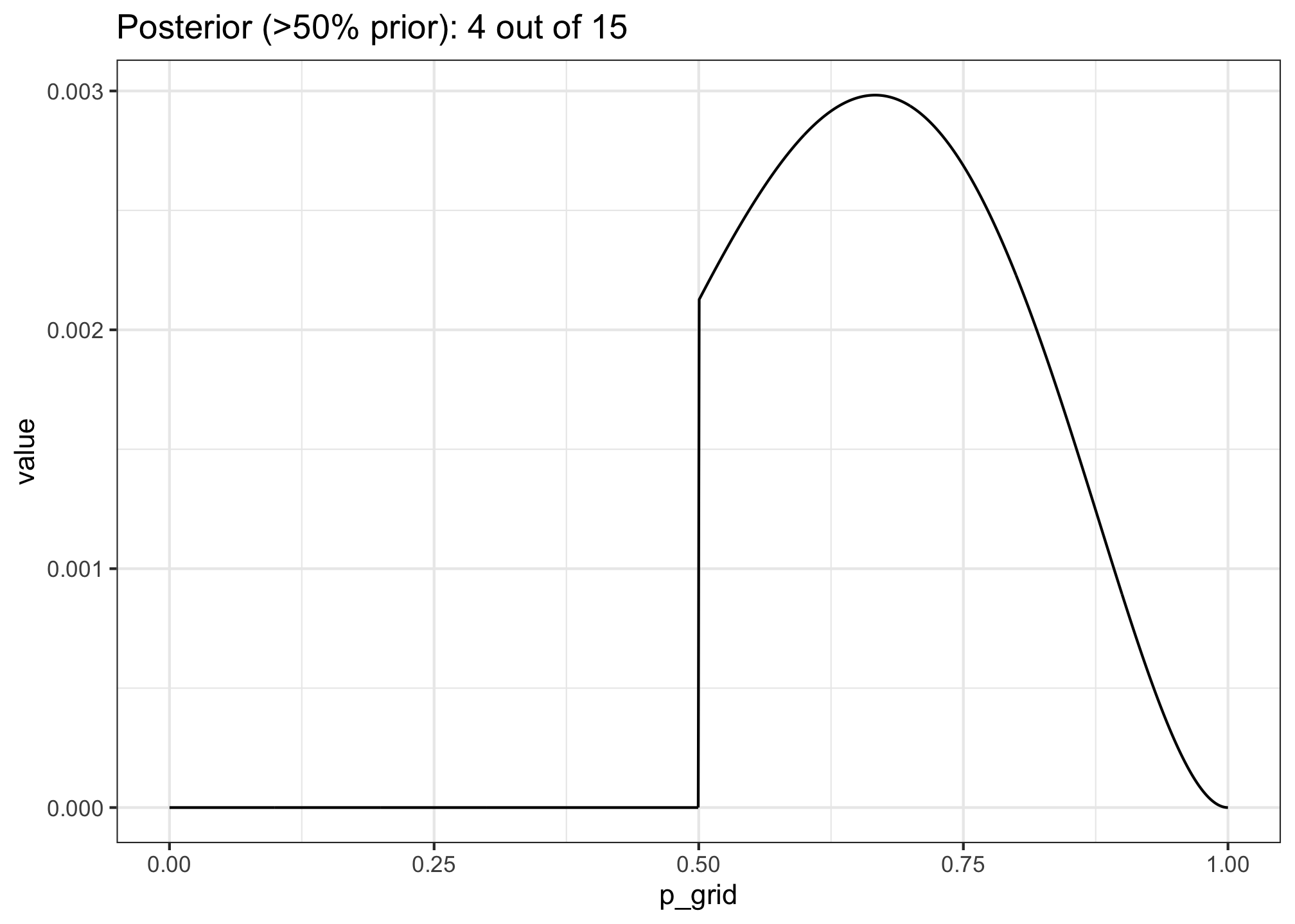
- Now suppose the data are 4 water and 2 land. Compute the posterior again, but this time use a prior that is zero below p = 0.5 and a constant above p = 0.5. This corresponds to prior information that a majority of the Earth’s surface is water. Compare the new posterior with the previous posterior (flat)
# how many grid points would you like?
n <- 1000
n_success <- 4
n_trials  <- 6

d <-
  tibble(p_grid = seq(from = 0, to = 1, length.out = n)) %>%
  mutate(prior = if_else(p_grid > 0.5, 0.3, 0)) %>%
  mutate(likelihood = dbinom(n_success, size = n_trials, prob = p_grid)) %>%
  mutate(posterior = (likelihood * prior) / sum(likelihood * prior))

d %>%
  pivot_longer(-p_grid) %>%
  filter(name == "posterior") %>%
  ggplot(aes(x = p_grid, y = value)) +
  geom_line() +
  ggtitle("Posterior (>50% prior): 4 out of 15") +
  theme_bw()
Package versions
sessionInfo()
## R version 4.1.1 (2021-08-10)
## Platform: aarch64-apple-darwin20 (64-bit)
## Running under: macOS Monterey 12.1
##
## Matrix products: default
## BLAS:   /Library/Frameworks/R.framework/Versions/4.1-arm64/Resources/lib/libRblas.0.dylib
## LAPACK: /Library/Frameworks/R.framework/Versions/4.1-arm64/Resources/lib/libRlapack.dylib
##
## locale:
## [1] en_US.UTF-8/en_US.UTF-8/en_US.UTF-8/C/en_US.UTF-8/en_US.UTF-8
##
## attached base packages:
## [1] parallel  stats     graphics  grDevices datasets  utils     methods
## [8] base
##
## other attached packages:
##  [1] forcats_0.5.1        stringr_1.4.0        dplyr_1.0.7
##  [4] purrr_0.3.4          readr_2.0.2          tidyr_1.1.4
##  [7] tibble_3.1.6         tidyverse_1.3.1      rethinking_2.21
## [10] cmdstanr_0.4.0.9001  rstan_2.21.3         ggplot2_3.3.5
## [13] StanHeaders_2.21.0-7
##
## loaded via a namespace (and not attached):
##  [1] matrixStats_0.61.0   fs_1.5.0             lubridate_1.8.0
##  [4] httr_1.4.2           tensorA_0.36.2       tools_4.1.1
##  [7] backports_1.4.1      bslib_0.3.1          utf8_1.2.2
## [10] R6_2.5.1             DBI_1.1.1            colorspace_2.0-2
## [13] withr_2.4.3          tidyselect_1.1.1     gridExtra_2.3
## [16] prettyunits_1.1.1    processx_3.5.2       compiler_4.1.1
## [19] rvest_1.0.2          cli_3.1.0            xml2_1.3.2
## [22] labeling_0.4.2       bookdown_0.24        posterior_1.1.0
## [25] sass_0.4.0           scales_1.1.1         checkmate_2.0.0
## [28] mvtnorm_1.1-3        callr_3.7.0          bsplus_0.1.3
## [31] digest_0.6.29        rmarkdown_2.11       base64enc_0.1-3
## [34] pkgconfig_2.0.3      htmltools_0.5.2      dbplyr_2.1.1
## [37] fastmap_1.1.0        highr_0.9            readxl_1.3.1
## [40] rlang_0.4.12         rstudioapi_0.13      shape_1.4.6
## [43] jquerylib_0.1.4      farver_2.1.0         generics_0.1.1
## [46] jsonlite_1.7.2       distributional_0.2.2 inline_0.3.19
## [49] magrittr_2.0.1       loo_2.4.1            Rcpp_1.0.7
## [52] munsell_0.5.0        fansi_0.5.0          abind_1.4-5
## [55] lifecycle_1.0.1      stringi_1.7.6        yaml_2.2.1
## [58] MASS_7.3-54          pkgbuild_1.3.1       grid_4.1.1
## [61] crayon_1.4.2         lattice_0.20-44      haven_2.4.3
## [64] hms_1.1.1            knitr_1.36           ps_1.6.0
## [67] pillar_1.6.4         uuid_1.0-3           codetools_0.2-18
## [70] stats4_4.1.1         reprex_2.0.1         glue_1.6.0
## [73] evaluate_0.14        blogdown_1.5         modelr_0.1.8
## [76] renv_0.14.0          RcppParallel_5.1.4   tzdb_0.1.2
## [79] vctrs_0.3.8          cellranger_1.1.0     gtable_0.3.0
## [82] assertthat_0.2.1     xfun_0.28            mime_0.12
## [85] broom_0.7.9          coda_0.19-4          ellipsis_0.3.2
## [88] downloadthis_0.2.1   xaringanExtra_0.5.5